Evanescent Operators, Finite Renormalization, and RG Closure

An evanescent operator is nonzero in the dimension used by a regulator but vanishes after projection to a specified integer dimension. It therefore represents no additional four-dimensional interaction, yet it can be indispensable during subtraction: an ultraviolet pole multiplying an $O(\epsilon)$ evanescent projection leaves a finite physical term. The safe procedure is to renormalize a closed $d$-dimensional operator column, impose a finite prescription for its evanescent directions, and only then project to the physical basis.

This page uses $d=4-2\epsilon$, the operator convention $O_0=Z_OO$, and $g\equiv\alpha/(4\pi)$. It constructs the physical–evanescent mixing system and computes the finite shift caused by $E\to E+\epsilon aQ$. The example is algebraic: the number $z$ denotes a pole residue obtained from a normalized loop calculation, so the derivation applies to any four-fermion sector with that one-loop block.

Required background. Fierz Relations and Dimension-Specific Identities supplies the four-dimensional relation that defines the example’s evanescent direction. Operator Mixing and Renormalization Matrices fixes $O_0=Z_OO$ and the meaning of matrix entries. Dimensional Regularization and Minimal Subtraction fixes $d=4-2\epsilon$ and the pole convention.

Helpful background. Renormalization Conditions, Schemes, and Finite Parts explains why a finite operator normalization is a scheme choice rather than new physics.

Evanescent completion of a physical basis

Let $\Pi_4$ denote the projection that applies the declared four-dimensional Lorentz and spinor identities after renormalization. A physical operator $Q$ has a nonzero class $\Pi_4Q$, whereas an evanescent operator obeys

$$\Pi_4E=0.$$

This statement is weaker than $E=0$ in $d$ dimensions. For the four-fermion pair on the preceding page,

$$\begin{aligned} Q&=Q_S,\\ E_F&=Q_X-Q_S, \end{aligned}$$

and $\Pi_4E_F=0$ follows from the chiral Fierz identity. Before the projection, $E_F$ is an independent tensor structure. More generally a $d$-dimensional Dirac chain can be decomposed as

$$X(d)=f(\epsilon)Q+E, \qquad f(\epsilon)=f_0+\epsilon f_1+\cdots.$$

Only $f_0$ is fixed by the four-dimensional identity. Moving an $O(\epsilon)$ term between $f(\epsilon)Q$ and $E$ gives the equally valid definition

$$E^{(a)}=E+\epsilon aQ.$$

The parameter $a$ is part of the subtraction convention. It is harmless only when matching coefficients, anomalous dimensions, and matrix elements are all translated with it. Herrlich and Nierste display this freedom for explicit four-quark Dirac structures and derive its physical-sector scheme transformation in Herrlich and Nierste 1995, §§ 2–4, preprint pp. 3–11, Open PDF.

Evanescent operators are distinct from equation-of-motion operators, total derivatives, and BRST-exact operators. Those directions are removed by equations of motion, integration and boundary conditions, or a cohomological quotient; an evanescent direction is removed by an integer-dimensional algebraic projection. A calculation can require several of these sectors simultaneously.

Renormalization must close before projection

Order the renormalized column as physical and evanescent operators,

$$O= \begin{pmatrix} Q\\ E \end{pmatrix}, \qquad O_0=Z_OO.$$

At one loop a generic closed block has the form

$$Z_O = \mathbf1 +g\left[ \frac1\epsilon \begin{pmatrix} z_{QQ}&z_{QE}\\ z_{EQ}&z_{EE} \end{pmatrix} + \begin{pmatrix} r_{QQ}&r_{QE}\\ r_{EQ}&r_{EE} \end{pmatrix} \right] +O(g^2).$$

The pole matrix is determined by divergent projected insertion vertices. The finite matrix includes any prescription imposed on the evanescent sector. A widely useful condition is

$$\lim_{\epsilon\to0} \langle f|E(\mu)|i\rangle=0$$

for the declared physical external states and through the calculated order. Achieving it generally requires a finite counterterm proportional to physical operators. With a consistent all-orders extension, the anomalous-dimension matrix in the same $(Q,E)$ ordering can be chosen as

$$\gamma= \begin{pmatrix} \gamma_{QQ}&\gamma_{QE}\\ 0&\gamma_{EE} \end{pmatrix}.$$

With $\mathcal D O=-\gamma O$, the lower-left zero makes the evanescent subspace invariant: an $E$ insertion does not acquire a physical component under RG evolution. The physical quotient then evolves with $\gamma_{QQ}$ once renormalized evanescent matrix elements are projected away. This does not mean that the evanescent sector may be omitted: physical insertions can generate evanescent counterterms, and their finite projections affect higher-order physical anomalous dimensions and matching. Dugan and Grinstein prove the decoupling construction while retaining the enlarged tower in Dugan and Grinstein 1991, pp. 239–244.

A new evanescent tensor can appear when an existing one is inserted into a loop. Formally this produces an infinite tower, but at any fixed perturbative order only the structures reachable to that order are needed. Closure means that every ultraviolet pole generated by the chosen insertions and projectors expands in the retained $d$-dimensional column.

The workflow below places that closure check before translation to a physical representative. Inspect the fourth stage: its $d$-dimensional block is part of the basis result, not an optional correction to a four-dimensional count.

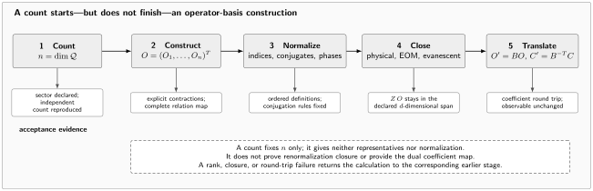
An operator-basis result is a five-stage package. Counting fixes $n=\dim\mathcal Q$; construction supplies explicit contractions and relations; normalization fixes ordering, conjugation, and phases; closure enlarges the $d$-dimensional renormalization space when EOM or evanescent operators are required; and translation applies $O'=BO$ with the dual coefficient map $C'=B^{-T}C$. The lower row states the acceptance evidence at each stage. A count alone is neither an explicit basis nor proof of RG closure. The diagram is schematic and not to scale.

First application: a finite shift in a two-operator sector

Retain the pole entry that mixes the renormalized evanescent representative into the bare physical operator. In scheme $A$, suppose the normalized one-loop calculation gives

$$Q_0 =Q_A+g\frac{z}{\epsilon}E_A+O(g^2).$$

The remaining row and diagonal poles are needed in a complete calculation but do not affect this finite-shift benchmark. Now choose scheme $B$ by changing the evanescent definition,

$$E_B=E_A+\epsilon aQ_A.$$

Substitute $E_A=E_B-\epsilon aQ_A$ into the same bare relation:

$$\begin{aligned} Q_0 &=Q_A+g\frac{z}{\epsilon} \left(E_B-\epsilon aQ_A\right)+O(g^2)\\ &=(1-gza)Q_A +g\frac{z}{\epsilon}E_B+O(g^2). \end{aligned}$$

The $1/\epsilon$ pole has multiplied the $\epsilon aQ_A$ change and produced the finite term $-gzaQ_A$. Define the minimally normalized physical representative in scheme $B$ by

$$\boxed{Q_B=(1-gza)Q_A+O(g^2)}.$$

Then the bare relation again has pure-pole form,

$$Q_0=Q_B+g\frac{z}{\epsilon}E_B+O(g^2).$$

This is the requested finite scheme shift. Its sign follows from the declared choices $O_0=Z_OO$ and $E_B=E_A+\epsilon aQ_A$; reversing either convention reverses the displayed intermediate sign.

Now pair the operator with its Wilson coefficient. In the four-dimensional physical projection,

$$\mathcal L_{\rm eff} \supset C_AQ_A=C_BQ_B.$$

Because the coefficient is a dual coordinate,

$$C_B=(1+gza)C_A+O(g^2).$$

The renormalized matrix element transforms oppositely,

$$\langle Q_B\rangle =(1-gza)\langle Q_A\rangle+O(g^2).$$

Their product therefore passes the physical check:

$$\boxed{ C_B\langle Q_B\rangle =C_A\langle Q_A\rangle+O(g^2) }.$$

The cancellation is not an argument that $a$ or $z$ can be forgotten. A Wilson coefficient computed with definition $a_A$ and a matrix element computed with $a_B$ differ at the same order by the uncancelled finite term $gz(a_B-a_A)$. At next-to-leading order the same finite map also changes the physical anomalous-dimension matrix; matching, running, and matrix elements must use one convention or explicit conversion formulae.

A complete scheme declaration

An evanescent prescription must state more than the name of a physical basis. Record the $d$-dimensional gamma and metric algebra, the $\gamma_5$ prescription if chiral tensors occur, every evanescent definition including its $O(\epsilon)$ physical part, the operator ordering and normalization, the subtraction scheme, and the finite condition imposed on renormalized evanescent matrix elements. Also retain the physical–evanescent pole blocks through the loop order at which they first affect the physical result.

The evanescent fixture and exact quotient-basis round trip should reproduce both algebraic identities

$$Q_0=Q_A+g\frac z\epsilon E_A =Q_B+g\frac z\epsilon E_B+O(g^2)$$

and

$$(1+gza)(1-gza)=1+O(g^2)$$

without floating-rank decisions.

The operator-basis reproducibility record

For an evanescent calculation, the renormalization-data, dimensional-identity, coefficient-map, and round-trip rows are essential. Use the chapter-wide record unchanged.

Record	Declare before reduction	Verification retained with the result
Field content and order	Spacetime dimension, dynamical fields, exact symmetries, charges, EFT grading, and truncation	Every candidate and relation has the declared labels and order
Flavor, Hermiticity, and CP	Flavor-index ranges, conjugation rule, coefficient reality conditions, and CP convention	Conjugate completion and independent real parameter count agree
Operator definition	Ordered names, explicit index contractions, derivative placement, signs, and normalization factors	Each symbolic or numerical column maps to one unambiguous operator
Renormalization data	Regulator, subtraction scheme, gauge convention when relevant, renormalization scale $\mu$, and coupling definitions	Coefficients and matrix elements use the same scheme and scale
Dimensional identities	Dimension used for Lorentz and spinor algebra, $\gamma_5$ prescription when present, and evanescent-operator definitions	The renormalized basis closes before any four-dimensional projection
Redundancy generators	IBP currents and boundary conditions, lower-order EOM, field maps, and algebraic identities	Every relation row is reproducible from a displayed generator
Basis map	Candidate and reduced dimensions, matrix orientation, exact rank, pivots, and representative ordering	Nullities and ranks satisfy the quotient dimension and no pivot is tolerance-dependent
Coefficient map	Dual transformation, transpose convention, finite shifts, and perturbative order	$C^TO$ is unchanged through the retained order
Implementation identity	Source or notebook version, dependency versions, input hash, and output checksum	A clean rerun reproduces the ordered map and checksum
Round trip and physics	Forward and inverse maps on the common subspace plus one amplitude, correlator, or counting benchmark	The round trip is the identity and the benchmark is basis independent to the stated tolerance

For the two-operator benchmark, retain the ordered column $(Q,E)$, the definition $E_B=E_A+\epsilon aQ_A$, the pole residue $z$, the finite map $Q_B=(1-gza)Q_A$, and the inverse coefficient map. The invariant product $C\langle Q\rangle$ is the minimum physical round trip.

Common pitfalls

Setting an evanescent operator to zero inside a divergent graph. The projection $\Pi_4E=0$ is applied after subtraction. Before then, $E/\epsilon$ can carry a finite physical projection.

Keeping poles but omitting the finite evanescent counterterm. A renormalized evanescent insertion need not have vanishing four-dimensional matrix elements automatically. State and impose the finite condition used to define it.

Changing $E$ without translating coefficients and matrix elements. The replacement $E\to E+\epsilon aQ$ changes the finite normalization of $Q$. Combining ingredients from different definitions leaves a spurious scheme dependence.

Assuming one evanescent tensor closes every loop order. Insertions can generate new Dirac structures. Test closure at the target order and extend the tower as needed.

Leaving $\gamma_5$ implicit. Chiral dimensional algebra is prescription dependent. The evanescent definitions and any finite symmetry-restoring renormalization must use the same prescription.

Exercises

Suppose the scheme-$A$ pole is $Q_0=Q_A+2gE_A/\epsilon$ and choose $E_B=E_A-3\epsilon Q_A$. Find $Q_B$, $C_B$, and verify the coefficient–matrix-element product through order $g$.

Solution

Here $z=2$ and $a=-3$, so $gza=-6g$. Therefore

$$Q_B=(1+6g)Q_A, \qquad C_B=(1-6g)C_A.$$

Since $\langle Q_B\rangle=(1+6g)\langle Q_A\rangle$,

$$C_B\langle Q_B\rangle =(1-6g)(1+6g) C_A\langle Q_A\rangle =C_A\langle Q_A\rangle+O(g^2).$$

Why does the condition $\langle E\rangle_{d=4}=0$ not justify deleting $E$ from the counterterm basis?

Solution

The condition concerns a renormalized physical projection. Divergent off-shell insertion vertices are computed before that projection and can contain independent $d$-dimensional tensors proportional to $E$. Moreover, an $O(\epsilon)$ physical projection of $E$ multiplied by a $1/\epsilon$ pole is finite. Removing $E$ before subtraction therefore loses a local finite contribution and prevents the enlarged system from closing.

References

• Dugan, Michael J., and Benjamin Grinstein. 1991. “On the Vanishing of Evanescent Operators.” Physics Letters B 256 (2): 239–244. DOI.

• Herrlich, Stefan, and Ulrich Nierste. 1995. “Evanescent Operators, Scheme Dependences and Double Insertions.” Nuclear Physics B 455 (1–2): 39–58. DOI. Open PDF.