Scale Independence and the Callan–Symanzik Equation

Renormalized Green functions depend on the arbitrary subtraction scale $\mu$, even though the bare theory does not. That apparent contradiction is resolved by differentiating at fixed bare fields and parameters: the explicit $\mu$-dependence of loop logarithms is cancelled by the implicit running of renormalized couplings, masses and field normalizations. The resulting Callan–Symanzik equation is therefore a transport equation on the space of renormalized descriptions of one bare theory.

This page derives the equation for connected and one-particle-irreducible functions, solves it along characteristics, and checks it in the one-loop scalar four-point vertex. It also distinguishes the homogeneous fixed-bare equation from the inhomogeneous mass-insertion form used in analyses of broken scale invariance.

Required background. Renormalization Conditions, Schemes, and Finite Parts supplies the distinction between bare data and renormalized coordinates. The 1PI Effective Action and Mean-Field Equations supplies proper vertices and their relation to connected functions.

Helpful background. The Generating Functional fixes the source conventions behind the connected functions.

Fixed-bare differentiation

Use a real scalar theory in $d=4-2\epsilon$ only to make the bookkeeping concrete. Let

$$\phi_0=Z_\phi^{1/2}\phi, \qquad \lambda_0=\mu^{2\epsilon}Z_\lambda\lambda, \qquad m_0^2=Z_{m^2}m^2.$$

The local convention on this page is

$$\begin{aligned} \beta_d(\lambda,\epsilon) &\equiv \mu\frac{d\lambda}{d\mu}\bigg\rvert_0, & \beta(\lambda) &\equiv \lim_{\epsilon\to0}\beta_d, \\ \gamma_\phi &\equiv \frac12\mu\frac{d\ln Z_\phi}{d\mu}\bigg\rvert_0, & \gamma_{m^2} &\equiv -\mu\frac{d\ln m^2}{d\mu}\bigg\rvert_0. \end{aligned}$$

The subscript $0$ means that $\phi_0$, $\lambda_0$, $m_0^2$, and any other bare inputs are held fixed. In this convention $\beta_d=-2\epsilon\lambda+\beta(\lambda)$ in a mass-independent scheme, while

$$\mu\frac{dm^2}{d\mu}\bigg\rvert_0 =-\gamma_{m^2}m^2.$$

From here on, take the regulator-removal limit $\epsilon\to0$ and use the four-dimensional RG functions. At finite $\epsilon$, retain $\beta_d$ instead of $\beta$. For a renormalized function of fixed external momenta, fixed-bare differentiation becomes

$$\mathcal D \equiv \mu\frac{d}{d\mu}\bigg\rvert_0 = \mu\frac{\partial}{\partial\mu} +\beta\frac{\partial}{\partial\lambda} -\gamma_{m^2}m^2\frac{\partial}{\partial m^2}.$$

Additional running coordinates simply add their components to $\mathcal D$. The several-coupling geometry is developed on the coupled-flows page.

The sign of the field term depends on which renormalized object is differentiated. A connected $n$-point function and a proper $n$-point vertex obey

$$G_0^{(n)}=Z_\phi^{n/2}G_R^{(n)}, \qquad \Gamma_R^{(n)}=Z_\phi^{n/2}\Gamma_0^{(n)}.$$

Because both bare objects are independent of $\mu$ at fixed bare data,

$$\begin{aligned} (\mathcal D+n\gamma_\phi)G_R^{(n)}&=0, \\ (\mathcal D-n\gamma_\phi)\Gamma_R^{(n)}&=0. \end{aligned}$$

The opposite signs are not competing conventions: one factor of $Z_\phi^{1/2}$ multiplies each renormalized connected leg, whereas it multiplies each bare proper vertex when the effective action is re-expressed in terms of the renormalized classical field.

Renormalized object	Relation to the bare object	Homogeneous equation
Connected function $G_R^{(n)}$	$G_0^{(n)}=Z_\phi^{n/2}G_R^{(n)}$	$(\mathcal D+n\gamma_\phi)G_R^{(n)}=0$
Proper vertex $\Gamma_R^{(n)}$	$\Gamma_0^{(n)}=Z_\phi^{-n/2}\Gamma_R^{(n)}$	$(\mathcal D-n\gamma_\phi)\Gamma_R^{(n)}=0$

Equivalently, the 1PI effective action satisfies

$$\left[ \mathcal D -\gamma_\phi \int d^4x\, \phi(x)\frac{\delta}{\delta\phi(x)} \right]\Gamma_R[\phi]=0,$$

up to additive vacuum terms if the identity operator has not been included among the renormalized couplings. Collins obtains these equations directly from fixed-bare differentiation and proves that their coefficients remain finite after removing the regulator Collins 1984/2023, §§ 7.3.1–7.3.2, pp. 180–184.

The homogeneous Callan–Symanzik equation

For a scalar 1PI vertex, the result can be displayed as

$$\boxed{ \left[ \mu\frac{\partial}{\partial\mu} +\beta(\lambda)\frac{\partial}{\partial\lambda} -\gamma_{m^2}(\lambda)m^2\frac{\partial}{\partial m^2} -n\gamma_\phi(\lambda) \right] \Gamma_R^{(n)}=0. }$$

This is often called either the renormalization-group equation or the Callan–Symanzik equation. Usage varies. It is useful to reserve homogeneous RG equation for this fixed-bare $\mu$ derivative and inhomogeneous Callan–Symanzik equation for the momentum-dilatation equation with a mass-operator insertion derived below. The two forms contain the same scale information when all insertion counterterms are treated consistently.

The equation does not say that $\Gamma_R^{(n)}$ is separately independent of $\mu$ while $\lambda$, $m$, and $Z_\phi$ are frozen. Rather, it says that changing $\mu$ while moving the renormalized coordinates along the fixed-bare trajectory leaves the underlying theory unchanged. Callan’s original scalar analysis related this broken scale invariance to the renormalization group Callan 1970, §§ I–IV, pp. 1541–1547.

Characteristics and boundary data

Let $t=\ln(\mu'/\mu)$ and define the running coordinates by

$$\begin{aligned} \frac{d\bar\lambda}{dt} &=\beta(\bar\lambda), & \bar\lambda(0)&=\lambda, \\ \frac{d\ln\bar m^2}{dt} &=-\gamma_{m^2}(\bar\lambda), & \bar m^2(0)&=m^2. \end{aligned}$$

Along this curve, the 1PI equation reduces to an ordinary differential equation:

$$\frac{d}{dt} \Gamma_R^{(n)} \left( p_i;\bar\lambda(t),\bar m^2(t),\mu e^t \right) = n\gamma_\phi(\bar\lambda(t)) \Gamma_R^{(n)}.$$

Therefore

$$\begin{aligned} &\Gamma_R^{(n)} \left( p_i;\bar\lambda(t),\bar m^2(t),\mu e^t \right) \\ &\qquad= \exp\!\left[ n\int_0^t ds\, \gamma_\phi(\bar\lambda(s)) \right] \Gamma_R^{(n)}(p_i;\lambda,m^2,\mu). \end{aligned}$$

For a general multiplicatively evolving quantity satisfying

$$(\partial_t+\beta\partial_g+\gamma_F)F=0,$$

the same calculation gives

$$F(t_1,g_1) = \exp\!\left[ -\int_{t_0}^{t_1}dt\, \gamma_F(\bar g(t)) \right] F(t_0,g_0).$$

The boundary value is indispensable. RG functions determine transport, not the finite matching data at one reference scale. Collins formulates this characteristic solution and its boundary-condition dependence in Collins 1984/2023, § 7.3.3, pp. 184–185.

Read the figure from top to bottom. Panel (a) evolves all running coordinates of one bare theory; panel (b) transports supplied boundary data and checks it by re-expansion. Panel (c) is a separate asymptotically free example, not the scalar flow. The scale parameter $t$ is not physical time.

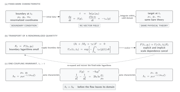
The figure uses a mass-independent scheme with $m^2>0$ and fixed external momenta. $g$ can be the vector of dimensionless couplings, and $m_*^2$ is a renormalized boundary value. The multiplicative $F$ follows the complete characteristic, with mass arguments suppressed. For $F=G_R^{(n)}$, $\gamma_F=n\gamma_\phi$; for $F=\Gamma_R^{(n)}$, $\gamma_F=-n\gamma_\phi$, giving the positive forward vertex exponent derived above. Complete observables are scale independent; finite-order predictions retain higher-order scale dependence. Panel (c) separately preserves $\Lambda_{\mathrm{RG}}$ in its one-loop domain. The diagram is schematic and not to scale.

The same content is available without the graphic:

Stage	Equation	Meaning and independent check
Fixed-bare path	$t=\ln(\mu_1/\mu_0)$, $d\bar g/dt=\beta(\bar g)$	The endpoints use different renormalized coordinates for one bare theory
Quantity transport	$U_F=\exp[-\int_{t_0}^{t_1}\gamma_F(\bar g(t))dt]$	Differentiating $U_FF_0$ returns $dF/dt=-\gamma_FF$
Fixed-order recovery	Expand $\bar g(t)$ and $U_F$ in the boundary coupling	The expansion must reproduce the explicit logarithms through the retained order
One-coupling invariant	$\beta=-b_0g^3$, $\Lambda=\mu e^{-1/(2b_0g^2)}$	$d\ln\Lambda/d\ln\mu=1+\beta/(b_0g^3)=0$
Domain	Perturbative flow and multiplicative evolution remain valid	Stop before strong coupling, thresholds, operator mixing, or an infrared singularity invalidates the equation used

The last row matters: solving a truncated differential equation exactly does not make its extrapolation exact. The construction of $\Lambda$ and the physical meaning of dimensional transmutation are developed on the running-couplings page.

One-loop scalar four-point check

Take the massless $\lambda\phi^4/4!$ theory at a nonexceptional symmetric Euclidean configuration with

$$P_s^2=P_t^2=P_u^2=Q^2>0.$$

Strip the overall sign convention from the proper vertex and call the remaining scalar coefficient $\mathcal F$, normalized so that its tree term is $\lambda$. In a mass-independent scheme its one-loop form is

$$\mathcal F(Q;\lambda,\mu) = \lambda +\lambda^2 \left[ c_{\rm sym} +\frac{3}{32\pi^2} \ln\frac{Q^2}{\mu^2} \right] +\mathcal O(\lambda^3).$$

The finite constant $c_{\rm sym}$ depends on the subtraction convention and the precise symmetric-point normalization. The logarithm’s coefficient is fixed by the three one-loop channels. With

$$\beta(\lambda) = \frac{3\lambda^2}{16\pi^2} +\mathcal O(\lambda^3), \qquad \gamma_\phi=\mathcal O(\lambda^2),$$

the explicit scale derivative is

$$\mu\frac{\partial\mathcal F}{\partial\mu} = -\frac{3\lambda^2}{16\pi^2} +\mathcal O(\lambda^3),$$

while the implicit coupling dependence gives

$$\beta(\lambda) \frac{\partial\mathcal F}{\partial\lambda} = +\frac{3\lambda^2}{16\pi^2} +\mathcal O(\lambda^3).$$

The two terms cancel. The $-4\gamma_\phi\mathcal F$ term begins at $\mathcal O(\lambda^3)$, and there is no mass derivative in this massless, nonexceptional check. Hence

$$\left( \mu\partial_\mu +\beta\partial_\lambda -4\gamma_\phi \right)\mathcal F =\mathcal O(\lambda^3).$$

This is cancellation through the calculated order, not exact scale independence of the truncated polynomial. Intriligator derives the one-loop scalar beta function by differentiating the bare minimal-subtraction coupling and records the same coefficient Intriligator 2007, lecture 15, pp. 1–2, PDF.

Choosing the boundary scale $\mu_0\simeq Q$ makes the boundary logarithm small. Solving the characteristic and re-expanding gives

$$\bar\lambda(Q) = \lambda(\mu_0) +\frac{3\lambda^2(\mu_0)}{16\pi^2} \ln\frac{Q}{\mu_0} +\mathcal O(\lambda^3),$$

which reproduces the logarithmic part of $\mathcal F$. Keeping the unexpanded running coupling sums a tower of leading logarithms; the conditions under which that improves a prediction belong to Large Logarithms and RG Improvement.

Mass insertions and the inhomogeneous form

The homogeneous equation changes $\mu$ while keeping external momenta fixed. A momentum dilatation can be exposed by combining it with dimensional analysis. Define

$$\gamma_m\equiv\frac12\gamma_{m^2}, \qquad \mathcal P\equiv \sum_i p_i^\mu\frac{\partial}{\partial p_i^\mu},$$

where the sum runs over independent external momenta. A scalar proper vertex in four dimensions has engineering dimension $d_n=4-n$, so

$$(\mathcal P+m\partial_m+\mu\partial_\mu-d_n) \Gamma_R^{(n)}=0.$$

Eliminating $\mu\partial_\mu$ with the homogeneous RG equation gives

$$\left[ \mathcal P-d_n -\beta\partial_\lambda +n\gamma_\phi \right] \Gamma_R^{(n)} = -(1+\gamma_m)m\partial_m \Gamma_R^{(n)}.$$

The right-hand side measures explicit breaking by the relevant mass deformation. In Euclidean scalar normalization,

$$S_E\supset \frac12m^2\int d^4x\,\phi^2(x),$$

so a mass derivative is represented schematically by a zero-momentum insertion,

$$\frac{\partial\Gamma_R^{(n)}}{\partial m^2} = \frac12 \int d^4x\, \Gamma_{R,[\phi^2]}^{(n)}(x;p_1,\ldots,p_n) +\text{local normalization terms}.$$

The qualification is essential. The composite operator $[\phi^2]$ must itself be renormalized. Power counting restricts its counterterms to operators of the same or lower canonical dimension Collins 1984/2023, § 6.4, pp. 149–150. In the four-dimensional, $\mathbb Z_2$-symmetric scalar theory, the lower-dimensional mixing includes the identity, with a dimension-two coefficient; there is no nonzero $\mathbb Z_2$-even scalar total derivative of dimension at most two to add. Total derivatives can enter more general operator bases when dimensions and symmetries permit them.

Coincident insertions also generate contact terms. The detailed insertion construction is on Renormalized Composite-Operator Insertions. Callan’s equation uses precisely such a soft mass insertion, while Symanzik’s small-distance analysis states the power-counting conditions behind the scaling limit Callan 1970, §§ I–III, pp. 1541–1545, Symanzik 1970, §§ 2–4, pp. 230–240.

At nonexceptional Euclidean momenta much larger than $m$, the insertion can be power suppressed, yielding the familiar approximately homogeneous short-distance equation. It need not be suppressed at exceptional momenta or when the massless limit creates an infrared singularity. Setting $m=0$ before checking infrared safety is therefore not a valid derivation of scale invariance.

Explicit, implicit, and residual scale dependence

For any renormalized quantity, a scale derivative should be decomposed before it is interpreted:

$$\underbrace{ \mu\frac{dF}{d\mu}\bigg\rvert_0 }_{\text{fixed-bare total}} = \underbrace{ \mu\frac{\partial F}{\partial\mu} }_{\text{explicit logarithms}} + \underbrace{ \beta\partial_\lambda F -\gamma_{m^2}m^2\partial_{m^2}F }_{\text{running coordinates}}.$$

For field-normalized Green functions, the appropriate $\pm n\gamma_\phi F$ term must then be included according to the object table above. For an infrared-safe observable, external-field normalization cancels against the corresponding residues or operator factors, leaving a fixed-bare total derivative of zero in the exact theory.

For a result truncated at order $N$, define the RG residual by applying the same differential operator:

$$R_N \equiv (\mathcal D-n\gamma_\phi) \Gamma_{R,[N]}^{(n)}.$$

A consistent calculation has $R_N$ beginning at the first omitted order. A residual at an order already retained diagnoses a wrong logarithm, a missing counterterm, inconsistent running input, or a sign error. Moderate $\mu$ variation can probe the size of uncomputed terms, but it is not a probability distribution and cannot reveal every missing constant, new threshold, nonperturbative contribution, or infrared enhancement.

Common pitfalls

Holding the wrong quantities fixed. The partial derivative $\mu\partial_\mu$ at fixed renormalized $\lambda$ and $m$ is only the explicit part of the equation. The beta and mass terms arise because the bare theory—not the numerical renormalized coordinates—is held fixed.

Copying the field sign between objects. Connected functions and 1PI vertices carry opposite anomalous-dimension signs with the definitions used here. Start from the relevant bare–renormalized relation instead of memorizing an isolated formula.

Dropping the mass insertion without an infrared check. Large Euclidean momentum can suppress a soft mass insertion, but exceptional momentum or a singular massless limit can defeat that argument. State the kinematic regime before using a homogeneous scaling law.

Treating characteristic evolution as a boundary prediction. Beta functions and anomalous dimensions transport already matched data. They do not determine finite constants, threshold matching coefficients, or the normalization at the starting scale.

Calling a truncated answer scale independent. Exact fixed-bare scale independence becomes cancellation only through the retained order after truncation. The remaining scale dependence is a diagnostic whose interpretation depends on the calculation and its missing structures.

Where to continue

• Beta Functions, Running Masses, and Field Anomalous Dimensions derives the RG functions from counterterms and organizes their scheme dependence.
• Running Couplings and Dimensional Transmutation develops the invariant scale displayed in the figure and identifies the domain of the one-coupling solution.
• Large Logarithms and RG Improvement turns the characteristic solution into a controlled resummation workflow.

References

• Callan, Curtis G., Jr. “Broken Scale Invariance in Scalar Field Theory.” Physical Review D 2 (1970): 1541–1547. DOI.
• Collins, John C. Renormalization: An Introduction to Renormalization, the Renormalization Group, and the Operator-Product Expansion. Cambridge Monographs on Mathematical Physics. Cambridge: Cambridge University Press, 1984; open-access digital edition, 2023. DOI. Open PDF.
• Intriligator, Kenneth. “RG Equation: Beta and Gamma.” Lecture 15 outline, Physics 215B: Quantum Field Theory, University of California San Diego, 2 March 2007. PDF.
• Symanzik, Kurt. “Small Distance Behavior in Field Theory and Power Counting.” Communications in Mathematical Physics 18 (1970): 227–246. DOI.