The 1PI Effective Action and Mean-Field Equations

The one-particle-irreducible (1PI) effective action is the local Legendre reorganization of connected generating data. On a regulated in–out source neighborhood where the map from source to mean field is invertible, this page uses

$$\Gamma[\bar\phi] =W[J]-J\mathbin{\cdot}\bar\phi, \qquad \bar\phi=\frac{\delta W}{\delta J}.$$

Its first derivative returns the negative source, and its Hessian is the negative inverse of the connected-response Hessian. With the chapter’s Lorentzian convention $W^{(2)}=iG_{c,J}^{(2)}$, the exact relation is $\Gamma^{(2)}G_{c,J}^{(2)}=iI$. At zero source, $\Gamma$ is stationary at the exact in–out mean field. That statement is not a mean-field approximation, and its Feynman boundary data do not in general define a real causal initial-value equation.

Required background. Connected Correlators and Cumulants defines $W$, the source-dependent mean field, and the convention $W^{(2)}=iG_{c,J}^{(2)}$ used below.

The source–mean-field map

Keep the same regulator, normalized in–out state, integration cycle, source sign, and local logarithm branch used to define $W[J]$. For a real scalar source, write

$$J\mathbin{\cdot}\bar\phi \equiv \int \mathrm d^dx\,J(x)\bar\phi(x), \qquad \bar\phi_J(x) \equiv \frac{\delta W[J]}{\delta J(x)}.$$

The argument $\bar\phi$ is a c-number field configuration. It is often called the mean field, classical field, or background field; it is the argument of $\Gamma$, not a new path-integration variable. Its source response is

$$W^{(2)}(x,y) \equiv \frac{\delta^2W[J]}{\delta J(x)\delta J(y)} = \frac{\delta\bar\phi_J(x)}{\delta J(y)}.$$

At a finite regulator, an ordinary local Legendre transform requires this response matrix to be nonsingular at the source under consideration. In a functional setting, one must additionally specify source and field spaces and require the corresponding linearized map to possess the inverse needed below. This is a local statement: it does not assert that every mean field comes from one globally unique source.

The local Legendre transform

On such a branch, solve locally for $J=J[\bar\phi]$ and define

$$\Gamma[\bar\phi] \equiv W[J[\bar\phi]] -J[\bar\phi]\mathbin{\cdot}\bar\phi.$$

The sign is fixed by direct variation. Because $\delta W=\bar\phi\mathbin{\cdot}\delta J$,

$$\begin{aligned} \delta\Gamma &= \bar\phi\mathbin{\cdot}\delta J -\bar\phi\mathbin{\cdot}\delta J -J\mathbin{\cdot}\delta\bar\phi \\ &=-J\mathbin{\cdot}\delta\bar\phi. \end{aligned}$$

Therefore

$$\frac{\delta\Gamma[\bar\phi]}{\delta\bar\phi(x)} =-J(x), \qquad W[J] =\Gamma[\bar\phi_J]+J\mathbin{\cdot}\bar\phi_J.$$

The source labels an off-shell configuration through $J=-\Gamma^{(1)}$. Removing it gives the exact source-free mean-field equation

$$\left. \frac{\delta\Gamma}{\delta\bar\phi(x)} \right|_{\bar\phi=\bar\phi_0} =0, \qquad \bar\phi_0 =\left.\frac{\delta W}{\delta J}\right|_{J=0}.$$

Calling this a “mean-field equation” describes its variable, not an approximation scheme. Approximation enters only after $\Gamma$ itself is truncated or estimated. The Lorentzian derivation with this same Legendre sign is given in Schwartz 2014, § 34.1.2, pp. 737–740.

The two Hessians invert each other

Differentiate $\Gamma^{(1)}(x)=-J(x)$ with respect to $\bar\phi(z)$:

$$\Gamma^{(2)}(x,z) = -\frac{\delta J(x)}{\delta\bar\phi(z)}.$$

Composing this derivative with the response $W^{(2)}=\delta\bar\phi/\delta J$ gives

$$\int \mathrm d^dz\, \Gamma^{(2)}(x,z)W^{(2)}(z,y) =-\delta^{(d)}(x-y).$$

When the inverse is two-sided, the reverse composition also holds:

$$\int \mathrm d^dz\, W^{(2)}(x,z)\Gamma^{(2)}(z,y) =-\delta^{(d)}(x-y).$$

Thus, in operator notation,

$$\Gamma^{(2)} =-\bigl(W^{(2)}\bigr)^{-1}.$$

The physical connected two-point function is not $W^{(2)}$ under the present Lorentzian convention. Since

$$G_{c,J}^{(2)}=-iW^{(2)}, \qquad W^{(2)}=iG_{c,J}^{(2)},$$

the corresponding inverse-kernel identity is

$$\Gamma^{(2)}G_{c,J}^{(2)}=iI, \qquad \Gamma^{(2)} =i\bigl(G_{c,J}^{(2)}\bigr)^{-1}.$$

Every factor in these products carries the same regulator, field indices, operator domain, and in–out boundary prescription. Replacing $iI$ by $I$ would mix the physical correlator with the $W$ Hessian.

The following map gathers the operations and the conditions that make them reversible. Read the central path from top to bottom, then inspect the dashed qualifications: local invertibility and Feynman boundary data are part of the statement, not optional annotations.

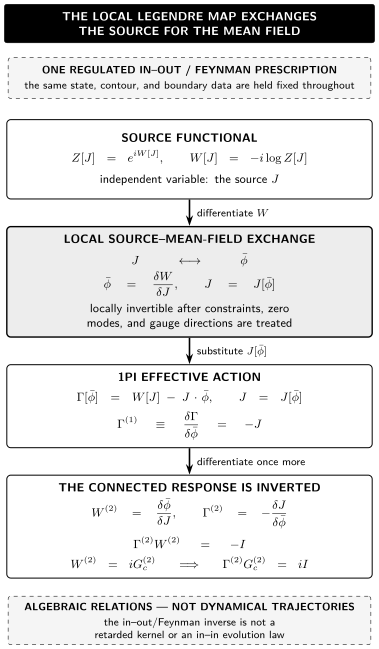
Local in–out Legendre map (schematic, not to scale). With normalized $Z$, $W=-i\log Z$, $\bar\phi=\delta W/\delta J$, and $\Gamma=W-J\cdot\bar\phi$ on a branch where $W^{(2)}$ is invertible, the Hessians obey $\Gamma^{(2)}W^{(2)}=-I$, equivalently $\Gamma^{(2)}G_{c,J}^{(2)}=iI$. The drawing suppresses the background-source subscript $J$ on $G_c^{(2)}$. Every kernel retains the same Feynman boundary prescription; the arrows denote functional operations, not causal propagation.

The same content is available without the image.

Stage	Operation	Qualification
$Z\to W$	$W=-i\log Z$	Use the normalized functional and a fixed local logarithm branch
$W\to\bar\phi$	$\bar\phi=W^{(1)}$ and $W^{(2)}=iG_{c,J}^{(2)}$	The derivative is an in–out/Feynman response, not a retarded one
$\bar\phi\leftrightarrow J$	Invert the source–mean-field map locally	$W^{(2)}$ must be invertible on the declared regulated space
$(W,J,\bar\phi)\to\Gamma$	$\Gamma=W-J\cdot\bar\phi$	The site convention gives $\Gamma^{(1)}=-J$
Hessian relation	$\Gamma^{(2)}W^{(2)}=-I$, hence $\Gamma^{(2)}G_{c,J}^{(2)}=iI$	Both compositions use the same domain and boundary prescription

Why the vertices are one-particle irreducible

About a source-free stationary configuration $\bar\phi_0$, the formal vertex expansion is

$$\Gamma[\bar\phi_0+\varphi] = \Gamma[\bar\phi_0] +\sum_{n\ge2}\frac{1}{n!} \,\Gamma^{(n)}[\bar\phi_0]\mathbin{\cdot}\varphi^n.$$

Here the dot includes all spacetime integrations and internal-index contractions. In perturbation theory, $\Gamma^{(n)}$ is the proper $n$-point kernel: its contributing connected diagrams cannot be separated into two nontrivial pieces by cutting one internal propagator line. “1PI” is always relative to the fields and sources that were Legendre transformed.

The Legendre definition is conceptually prior to the diagrammatic label. Differentiating the inverse-Hessian relation already shows how connected data are reconstructed as trees of proper vertices joined by full response kernels. For example, in the present sign convention,

$$\begin{aligned} W^{(3)}(x,y,z) &= \int \mathrm d^da\,\mathrm d^db\,\mathrm d^dc \\ &\quad\times W^{(2)}(x,a)W^{(2)}(y,b)W^{(2)}(z,c) \\ &\quad\times \Gamma^{(3)}(a,b,c). \end{aligned}$$

Using $G_{c,J}^{(3)}=-W^{(3)}$ and $W^{(2)}=iG_{c,J}^{(2)}$, the same relation in terms of physical connected correlators is

$$G_{c,J}^{(3)} = i\bigl(G_{c,J}^{(2)}\bigr)^{\otimes3} \mathbin{\cdot}\Gamma^{(3)}.$$

The tensor-power notation denotes the same three external convolutions displayed in the preceding equation, with every kernel evaluated at the corresponding source and mean field.

At fourth order, one obtains a term with one $\Gamma^{(4)}$ vertex and terms with two $\Gamma^{(3)}$ vertices joined by a full line; higher orders continue the tree pattern. This removes one-particle-reducible compositions from the vertex kernels while retaining them in connected correlators. Schwartz derives the equivalence between the Legendre functional and the sum of 1PI vertices in Schwartz 2014, § 34.1.2, pp. 739–740. Zinn-Justin displays the inverse-kernel and connected-tree reconstruction in a Euclidean convention in which $\Gamma_{\mathrm E}=J\cdot\phi-W_E$; translating that algebraic sign gives the formulas above Zinn-Justin 2021, § 7.7, pp. 141–143.

The exact $\Gamma$ is generally nonlocal and may be complex. Its perturbative expansion does not by itself establish convergence or a nonperturbative definition, and it is not the same object as a Wilsonian action or a 2PI functional.

The exact free-scalar check

Take the regulated quadratic action to be

$$S_{0,F}[\phi] = -\frac12\phi\mathbin{\cdot}P_F\mathbin{\cdot}\phi,$$

where $P_F$ is symmetric as a scalar bilinear kernel and includes the deformation that selects the Feynman boundary value. Assume it is invertible on the declared regulated space, with

$$G_F=P_F^{-1}=iD_F, \qquad P_FG_F=I, \qquad P_FD_F=-iI.$$

The normalized Gaussian connected functional is

$$W_0[J] =\frac12J\mathbin{\cdot}G_F\mathbin{\cdot}J, \qquad \bar\phi=G_FJ, \qquad J=P_F\bar\phi.$$

Substitution into the Legendre transform gives the whole free effective action:

$$\begin{aligned} \Gamma_0[\bar\phi] &= \frac12(P_F\bar\phi)\mathbin{\cdot}G_F \mathbin{\cdot}(P_F\bar\phi) -(P_F\bar\phi)\mathbin{\cdot}\bar\phi \\ &= -\frac12\bar\phi\mathbin{\cdot}P_F \mathbin{\cdot}\bar\phi. \end{aligned}$$

There is no source-independent term because the normalized choice has $Z_0[0]=1$ and hence $W_0[0]=0$. Differentiation gives

$$\Gamma_0^{(1)}=-P_F\bar\phi=-J, \qquad \Gamma_0^{(2)}=-P_F.$$

Both inverse relations now reduce to one-line checks:

$$\begin{aligned} \Gamma_0^{(2)}W_0^{(2)} &=(-P_F)G_F=-I, \\ \Gamma_0^{(2)}G_{c,0}^{(2)} &=(-P_F)D_F=iI. \end{aligned}$$

The sourced equation $-P_F\bar\phi=-J$ is therefore the same equation as $\bar\phi=G_FJ$. At $J=0$, it becomes $P_F\bar\phi_0=0$ with the selected Feynman boundary prescription; in the regulated vacuum sector with no zero mode, $\bar\phi_0=0$. The free calculation and inverse two-point check are worked in Schwartz 2014, § 34.1.3, pp. 740–741.

Local inversion, zero modes, and convex conjugates

The local transform fails wherever $W^{(2)}$ has no inverse on the declared space. Gauge directions, untreated global or infrared zero modes, and a singular response at a critical point are common causes. Depending on the problem, one may restrict or project the space, fix the gauge, retain a regulator or deformation, or treat the null sector separately. The transform can also cease to be defined where a zero or branch change of $Z[J]$ makes the chosen $W=-i\log Z$ singular.

Global invertibility is a separate question. Two distant sources can produce the same mean field even though $W^{(2)}$ is invertible on a neighborhood of each source; then each local branch is valid, but there is no single global function $J[\bar\phi]$ covering both. Local repairs and branch choices do not establish a global inverse without an additional argument.

There is a different global construction for a real Euclidean convex functional. In finite-dimensional notation, its convex conjugate is

$$\Gamma_E^{\mathrm{LF}}[\phi] = \sup_J\left\{ J\mathbin{\cdot}\phi-W_E[J] \right\}.$$

If $W_E$ is differentiable and the supremum is attained at a unique source $J(\phi)$, stationarity gives $\phi=\delta W_E/\delta J$. Wherever the conjugate is differentiable, $\delta\Gamma_E^{\mathrm{LF}}/\delta\phi=J(\phi)$, and the ordinary transform is recovered on that regular branch. The general supremum definition and its differentiable reduction are stated in Boyd and Vandenberghe 2004, § 3.3.1, p. 91; “Differentiable functions,” p. 95, official PDF.

This Euclidean sign is opposite to the site’s Lorentzian algebraic convention: Zinn-Justin writes $\Gamma_E+W_E-J\cdot\phi=0$ and hence $\Gamma_E^{(1)}=J$ Zinn-Justin 2021, § 7.7, pp. 141–143. The sign translation is not a Wick rotation. Analytic continuation between $W_E$ and the Lorentzian in–out functional supplies its own factors of $i$. Moreover, a generally complex Lorentzian $W[J]$ has no order relation from which to form the displayed real supremum, so Euclidean convexity must not be imported into the in–out problem.

In–out stationarity is not causal evolution

The source derivatives of $W$ retain the vacuum in–out/Feynman boundary prescription. Consequently, $W^{(2)}$ is a Feynman response kernel and $\Gamma^{(2)}$ is its inverse with the same boundary data. A source-dependent $\bar\phi_J$ and the exact $\Gamma$ can be complex, and $\Gamma^{(1)}=0$ is generally a nonlocal boundary-value equation rather than a retarded initial-value equation.

Real causal expectation-value evolution requires a closed-time-path, or in–in, generating functional with doubled sources and fields. Jordan’s construction explicitly contrasts expectation values with ordinary in–out amplitudes and establishes reality and causality through two-loop order, rather than asserting an unrestricted all-orders result Jordan 1986, abstract. The formulation and its boundary data are developed on In–Out versus In–In Expectation Values.

Common pitfalls

Dropping the Lorentzian factor. The $W$ Hessian and physical connected two-point function differ by $W^{(2)}=iG_{c,J}^{(2)}$. Therefore $\Gamma^{(2)}G_{c,J}^{(2)}=iI$, not $I$.

Treating “mean field” as an approximation. The equation $\Gamma^{(1)}=0$ is exact when $\Gamma$ is exact. Hartree, loop, derivative, and semiclassical approximations arise only after a truncation is chosen.

Assuming global invertibility. A nonsingular Hessian supports a local inverse on a stated space; it does not rule out distant branches, phase transitions, or null directions. Gauge redundancy must be handled before the ordinary inverse is used.

Equating distinct effective actions. The 1PI functional trades a linear source for its mean field. A Wilsonian action integrates out specified modes, while 2PI and higher effective actions Legendre-transform additional composite sources.

Reading an in–out equation causally. Feynman boundary data are not retarded boundary data. Changing the physical question requires changing the contour and generating functional, not merely relabeling the same Hessian.

Check your understanding

Use the success criteria and repair links to test the Legendre transform, inverse-Hessian relation, and scope claims.

Check	A successful response	Repair route
Retrieve the transform and source equation	States $\Gamma=W-J\cdot\bar\phi$ and derives $\Gamma^{(1)}=-J$	Local Legendre transform
Distinguish connected from 1PI	Says $W$ generates connected kernels, while $\Gamma$ generates proper kernels whose connected reconstructions are trees	Why the vertices are 1PI
Derive the inverse relation	Composes $\delta J/\delta\bar\phi$ with $\delta\bar\phi/\delta J$ and obtains both $-I$ products	The two Hessians
Diagnose a zero mode	Explains why $W^{(2)}v=0$ blocks the inverse along $v$ and names a justified restriction, projection, gauge fixing, or deformation	Local inversion and zero modes
Transfer the finite Gaussian	For $W=\tfrac12J^{\mathsf T}CJ$, obtains $\bar\phi=CJ$ and $\Gamma=-\tfrac12\bar\phi^{\mathsf T}C^{-1}\bar\phi$	Exact free-scalar check
Choose the next construction	Routes renormalized or Wilsonian work, 2PI truncations, and causal evolution to the appropriate later treatments	Where the construction continues

Where the construction continues

• Schwinger–Dyson Identities next derives exact regulated field-variation identities; the 1PI language is helpful but not required for that derivation.
• Renormalization and Effective Field Theory develops renormalized effective-action calculations, loop effective potentials, derivative expansions, and the Wilsonian comparison.
• 2PI and nPI Effective Actions develops bilocal sources, gap equations, and self-consistent truncations.
• In–Out versus In–In Expectation Values changes the contour when the target is a real causal expectation-value equation.

References

• Boyd, Stephen, and Lieven Vandenberghe. Convex Optimization. Cambridge: Cambridge University Press, 2004. Official book page.
• Jordan, R. D. “Effective Field Equations for Expectation Values.” Physical Review D 33 (1986): 444–454. DOI.
• Schwartz, Matthew D. Quantum Field Theory and the Standard Model. Cambridge: Cambridge University Press, 2014. DOI.
• Zinn-Justin, Jean. Quantum Field Theory and Critical Phenomena. 5th ed. Oxford: Oxford University Press, 2021. DOI.