

Coherent States and the Classical Limit
Within a chosen free-field Fock representation, a coherent state is a unitary displacement of the vacuum. Its annihilation-operator eigenvalues become the mode amplitudes of a classical Klein–Gordon solution, so every linear field expectation value follows that solution exactly. This is a useful but limited classical regime: displacement leaves the vacuum covariance unchanged, and only specified observables with sufficiently large means acquire small relative fluctuations. Large occupation, a classical-looking one-point function, or nearly orthogonal wave packets does not by itself establish decoherence or a measurement outcome.
The scope is a massive real scalar in a periodic spatial box of volume , with a finite inversion-symmetric mode set , the standard positive-frequency split, and the corresponding vacuum . Every sum and operator identity below is therefore an ordinary finite-oscillator statement. The page does not remove the regulator, assign a finite pointwise continuum variance, evolve coherent states through interactions, develop squeezing, or derive environment-induced decoherence.
Required background. Fock Space, Vacuum, and Particle Number supplies the selected scalar vacuum, the regulated oscillators, their occupation basis, and the free Hamiltonian used below.
A displacement of the vacuum defines a coherent state
Section titled “A displacement of the vacuum defines a coherent state”For each retained momentum, the regulated oscillators obey
Choose complex, dimensionless amplitudes and write
The multimode displacement operator and its coherent state are
The exponent is anti-Hermitian, so is unitary and the state is normalized. Because the commutator of the exponent with any is a scalar, the Baker–Campbell–Hausdorff series stops after its first commutator:
It follows immediately that
Thus a coherent state is a simultaneous normalizable eigenstate of all the annihilators, not an eigenstate of the Hermitian field or of the creation operators.
Here and below, normal ordering is relative to the same selected free Fock vacuum: creation operators are moved to the left of annihilation operators, and denotes the resulting order. Normal Ordering and Vacuum Terms explains why this operation is vacuum-relative. In the present calculation, set
The scalar commutator licenses the exact BCH factorization
Because , expanding gives the occupation expansion
where every runs over the nonnegative integers. The occupation probabilities therefore factorize:
Each mode has a Poisson distribution. Although contains arbitrarily high particle sectors, the exponential tail puts it in the domain of every polynomial in the finitely many number operators and in the domain of the regulated free Hamiltonian.
The coherent-state eigenvalue, Poisson, and normal-ordering properties are developed in Coleman 2019, § 8.5, pp. 171–173, and problem 4.2 with solution, pp. 175–180. The annihilator-eigenstate definition and multiparticle expansion are posed for relativistic bosons in Weinberg 1995, ch. 4, problem 3, p. 189. The single-oscillator construction and its minimum-dispersion check appear in Schwartz 2014, problem 2.7, p. 28.
Two coherent states are not generally orthogonal. For the finite amplitude vectors, abbreviate
Reordering their displacements gives
Therefore
Large phase-space separation makes the overlap exponentially small, but that fact will not be confused below with dynamical decoherence.
The field expectation is an exact classical free solution
Section titled “The field expectation is an exact classical free solution”With the inherited finite-box normalization, the regulated Heisenberg field is
where . Its coherent-state mean is
The conjugate term in the Hermitian field makes real. The amplitudes of annihilators at and are independent Fock-space coordinates; they do not themselves obey the reality condition imposed on a classical Fourier coefficient.
Every retained mode is on shell, hence
This is an exact equality for the regulated free theory, not an approximation. It also passes the dimensional check: the dimensionless multiplies , which has scalar-field dimension .
The same statement can be made in the Schrödinger picture. With
free evolution preserves the coherent-state family:
The amplitudes rotate mode by mode:
For any finite normally ordered polynomial ,
This exact factorization explains why coherent states reproduce classical wave amplitudes for an important class of observables. It does not extend to an arbitrarily ordered product without the commutator terms that carry vacuum fluctuations.
Displacement leaves the vacuum noise intact
Section titled “Displacement leaves the vacuum noise intact”Displacement shifts the field by a scalar while leaving its fluctuation operator unchanged:
Consequently the connected two-point function is exactly the vacuum one:
For one mode, introduce the canonical quadratures
Their coherent-state variances equal their vacuum variances:
Thus increasing the displacement does not reduce absolute quantum noise. It can reduce noise only relative to a growing mean. To state that test without using a point field, choose a real smearing function in the regulated box and define
Let and let be its vacuum variance. Under the amplitude scaling with ,
Whenever ,
The ratio falls as . At a node or cancellation where the mean vanishes, the same ratio is undefined or large even though the state has not suddenly become more quantum. Classicality claims must therefore name the observable, its resolution, the time interval, and a nonzero comparison scale.
Occupation and excitation energy supply independent checks. The Poisson factors give
Likewise,
Here . Subtracting the vacuum scalar changes the mean-energy reference but not the variance or any field fluctuation.
A localized packet makes the scaling test concrete
Section titled “A localized packet makes the scaling test concrete”Choose a packet center , a resolved carrier momentum , and a length that is large compared with the cutoff resolution and small compared with the box. On the finite momentum set, let
where is fixed by
This is a band-limited packet rather than a compactly supported field. When the retained grid resolves its width, its initial envelope is concentrated near with spatial width of order .
For a chosen mean occupation , set
Define the positive-frequency packet
The coherent-state mean field is then
Its envelope propagates and disperses according to the free relation. Increasing raises the classical field amplitude as without changing the vacuum covariance.
Introduce the packet frequency moments
The second moment is
The number and energy checks become
and
while its relative fluctuation is
For a narrow-band packet, is close to one. Taking therefore gives a one-percent number fluctuation and an approximately one-percent excitation-energy fluctuation. A real smearing function matched to a nonzero part of the packet has the same relative-field scaling. These estimates are controlled finite-mode statements; they do not assert exact spatial localization or a regulator-independent local variance.
The packet also defines one normalized oscillator,
Choose the overall phase of so that is real, and define
Then
Thus the aligned quadrature has the exact relative width . The coefficient differs from the number-fluctuation coefficient because and are different observables; both ratios scale as .
Classical mean behavior and decoherence are different tests
Section titled “Classical mean behavior and decoherence are different tests”The regulated coherent packet passes several precise checks, but each has a limited conclusion:
| Question | Exact coherent-state result | What must still be checked |
|---|---|---|
| Does the mean field follow classical dynamics? | Yes, for the free Klein–Gordon equation. | Interactions introduce fluctuation moments and can distort the state. |
| Are quantum fluctuations negligible? | Absolute linear-field noise equals vacuum noise; selected relative fluctuations fall at large displacement. | Name the smeared observable, resolution, nonzero scale, and time range. |
| Are separated packets distinguishable? | Their overlap is exponentially small in phase-space distance. | Small overlap does not turn a coherent superposition into a mixture. |
| Has decoherence occurred? | Not from free closed-system evolution alone. | Specify an environment or coarse graining and test the reduced state. |
The distinction is sharp for the superposition of opposite packets. Since
the components become nearly orthogonal at large occupation. Nevertheless, a normalized vector proportional to remains a pure coherent superposition under closed free evolution. Near-orthogonality supplies distinguishability, not an environment, a trace, or suppression of interference.
If a specified interaction correlates the packet branches with normalized environment states, the joint state can instead take the form
After tracing out the environment, the branch cross term is proportional to
Decoherence in this branch basis requires over the claimed interval. This mechanism and the corresponding reduced-density-operator calculation are exhibited in Zurek 2003, § IV.A.1 and Eqs. (4.9)–(4.13).
The figure puts the two tests beside each other without drawing an implication between them. Read the upper panel as a schematic one-standard-deviation contour for the finite packet mode, not as hard probability support or an unsmeared continuum field distribution. The lower panel begins only after a system–environment split and interaction have been supplied.
On a narrow screen, open the full-size scalable diagram and use the browser’s zoom and pan controls.
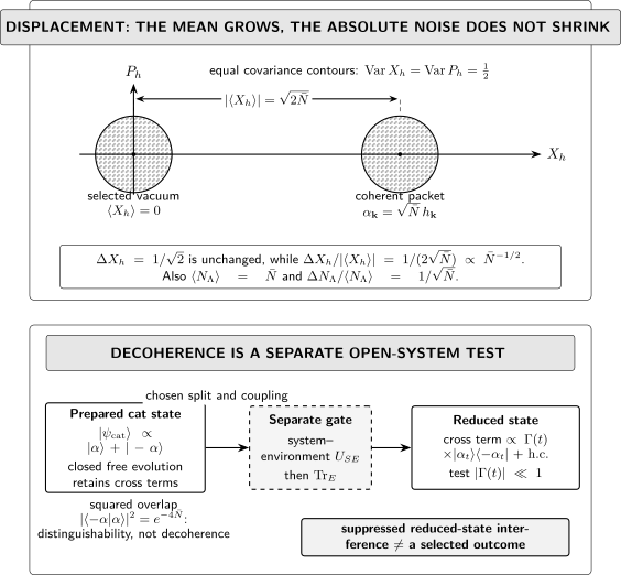
Schematic packet-mode phase space for a finite regulated free scalar, not to scale. Displacement changes the coherent mean by but leaves the covariance equal to the vacuum covariance, so noise in a nonzero aligned quadrature becomes small only relative to the mean. The lower panel is a separate open-system test: small opposite-packet overlap measures distinguishability, whereas reduced-state interference is suppressed only when is small after explicit system–environment dynamics and a partial trace. Such suppression does not select a unique outcome.
A genuine decoherence claim must at least identify:
- the system–environment split or the explicit coarse graining;
- the joint initial state and dynamics;
- the reduced density operator and the observables or basis in which interference is tested;
- the size and time dependence of the suppressed off-diagonal contribution; and
- stability, recoherence, and approximation errors over the claimed time interval.
Even a successful decoherence calculation does not by itself select a unique measurement outcome. System–Environment Splits and Influence Functionals develops reduced field dynamics, while Local Measurement Instruments in QFT treats outcomes and state updates. For cosmological squeezing and classicalization claims, continue to Decoherence and the Quantum-to-Classical Claim.
Two further contrasts prevent overstatement. A squeezed state can have large occupation and a vanishing mean while moving noise from one quadrature into another; large particle number is therefore not a universal classicality criterion. In an interacting theory, need not equal , so the one-point equation does not generally close on a classical field. Saddles and the Semiclassical Expansion develops the distinct path-integral expansion, and What an Interacting Lagrangian Does and Does Not Specify sets out the additional state, regulator, observable, and continuum data.
Common pitfalls
Section titled “Common pitfalls”Equating a classical one-point function with a classical state. The mean field follows the free classical equation exactly, but the state retains vacuum covariance and is a superposition of all number sectors. Classical behavior must be tested against specified observables and tolerances.
Using large occupation as the only criterion. A coherent packet has , but squeezed and number states show that occupation alone does not determine phase-space noise or a nonzero classical mean.
Dividing by a mean at a node. Pointwise relative fluctuation ratios become singular where an oscillating classical field crosses zero. Use a physically resolved smeared observable and an independently meaningful comparison scale.
Calling small overlap decoherence. Two macroscopic coherent packets can be almost orthogonal while their superposition remains pure. Decoherence requires a reduced-state or coarse-grained interference calculation with explicit dynamics.
Removing the regulator inside a variance formula. The finite-mode local variance is well defined, but the unsmeared continuum point field is distributional. Smear first and state the regulator limit separately.
Check your understanding
Section titled “Check your understanding”- Retrieval. Define and use it to show that .
- Distinction. Explain why an exact classical free-field one-point function does not imply zero quantum fluctuations or decoherence.
- Derivation. Starting from the factorized Poisson distribution, derive the mean and variance of and of .
- Failure diagnosis. Identify both errors in using at a field node and in using large occupation alone as a classicality test.
- Transfer. For with , recover the mean field and the two relative-fluctuation formulas for the localized packet.
- Handoff. Choose the appropriate continuation for open-system decoherence, local measurement outcomes, cosmological squeezing, and an interacting semiclassical expansion.
Answers and repair routes
Section titled “Answers and repair routes”- The exponent is anti-Hermitian, and . Multiplying by and using gives the eigenvalue equation. Repair the oscillator algebra at Fock Space, Vacuum, and Particle Number.
- Displacement changes the mean but leaves every connected linear-field two-point function equal to its vacuum value. Closed free evolution also preserves purity, so no environment has removed interference.
- Independent Poisson variables have mean and variance . Variances add across modes, and weighting each occupation by produces the stated energy mean and variance. Repair the occupation basis at Fock Space, Vacuum, and Particle Number.
- At a node the denominator vanishes although the absolute variance stays finite, so the ratio is not a stable diagnostic. Large occupation also omits phase, quadrature covariance, observable resolution, and reduced-state coherence; squeezed and number states are immediate counterexamples.
- Substitution gives , , and . Frequency weighting gives and .
- Use System–Environment Splits and Influence Functionals for reduced dynamics, Local Measurement Instruments in QFT for outcomes, Decoherence and the Quantum-to-Classical Claim for cosmological squeezing, and Saddles and the Semiclassical Expansion for the regulated path-integral expansion.
References
Section titled “References”- Coleman, Sidney. Lectures of Sidney Coleman on Quantum Field Theory. Edited by Bryan Gin-ge Chen, David Derbes, David Griffiths, Brian Hill, Richard Sohn, and Yuan-Sen Ting. Singapore: World Scientific, 2019. DOI.
- Schwartz, Matthew D. Quantum Field Theory and the Standard Model. Cambridge: Cambridge University Press, 2014. doi:10.1017/9781139540940.
- Weinberg, Steven. The Quantum Theory of Fields. Vol. I, Foundations. Cambridge: Cambridge University Press, 1995. doi:10.1017/CBO9781139644167.
- Zurek, Wojciech H. “Decoherence, Einselection, and the Quantum Origins of the Classical.” Reviews of Modern Physics 75 (2003): 715–775. DOI. Open PDF (arXiv v3).
Original QFT.org content:CC BY 4.0, unless an item supplies different terms. Third-party material retains its own terms.