Quantum Fields as Operator-Valued Distributions

A continuum quantum field is generally not an operator attached separately to every spacetime point. The symbol $\phi(x)$ is a distributional kernel: it becomes a controlled object only after it is paired with a smooth test function,

$$\phi(f) := \int \mathrm d^4x\, f(x)\phi(x).$$

Smearing suppresses arbitrarily short-wavelength contributions and gives the field a finite spacetime resolution. It does not make an unbounded field bounded, define a sharp-point operator, or license products such as $\phi(x)^2$. These distinctions are already present for the free scalar field. Hollands and Wald 2015, arXiv v2, § 1, p. 5 gives the precise structural motivation.

This page develops the physics-first layer needed before selecting a Wightman, algebraic, or microlocal axiom system. We work in four-dimensional Minkowski spacetime with metric $(+---)$ and natural units.

Helpful background. Test-Function Spaces, Distributions, Support, and Convergence supplies the test-function topology and distributional support used below. Convolution, Approximate Identities, and Poisson Summation supplies the regulated point-approximation language, while Locally Convex, Nuclear, and Rigged Hilbert Spaces supplies the stronger topological setting used in theorem-level formulations.

The controlled object is the smeared field

For localization, take

$$\mathcal D_{\mathrm{test}}(M) := C_c^\infty(M),$$

the smooth compactly supported complex-valued functions on spacetime. The support of $f$ specifies the finite region over which the field is sampled. On Minkowski spacetime one often extends a tempered field to the Schwartz space $\mathcal S(\mathbb R^4)$, whose rapid decrease is convenient in momentum space. These are different test-function spaces; neither should be substituted for the other without saying so.

Suppose a Hilbert-space representation has been chosen and $\mathscr D\subset\mathcal H$ is a common dense working domain. A useful minimal formulation of an operator-valued distribution is a linear assignment

$$\begin{aligned} \phi:\mathcal D_{\mathrm{test}}(M) &\longrightarrow \{\text{operators on }\mathscr D\},\\ f&\longmapsto\phi(f), \qquad \phi(f)\mathscr D\subseteq\mathscr D, \end{aligned}$$

such that, for every $\Psi,\Chi\in\mathscr D$,

$$f\longmapsto \langle\Psi,\phi(f)\Chi\rangle$$

is a scalar distribution. In particular, if $f_n\to0$ in the test-function topology, then every such matrix element tends to zero. For a sequence in $C_c^\infty$, this means that the supports eventually lie in one compact set and every derivative converges uniformly to zero there.

For a Hermitian scalar field the adjoint compatibility is

$$\phi(f)^*\big|_{\mathscr D} = \phi(\overline f).$$

This is a relation on the declared common domain, not an assertion that the maximal Hilbert-space adjoint has the same domain. Smearing controls ultraviolet behavior; it does not remove the domain questions of unbounded operators.

One can also postpone the Hilbert space entirely. In the algebraic formulation, $f\mapsto\phi(f)$ takes values in an abstract unital $*$-algebra. A state and its representation are chosen later, at which point the algebra elements become operators on a common dense domain. Hollands and Wald make both layers explicit in Hollands and Wald 2015, arXiv v2, § 2.1, pp. 11–14.

The map below separates the operation that smearing actually defines from two tempting but independent extensions. Inspect how support gives localization, then where the point limit and coincident product each encounter a barred implication.

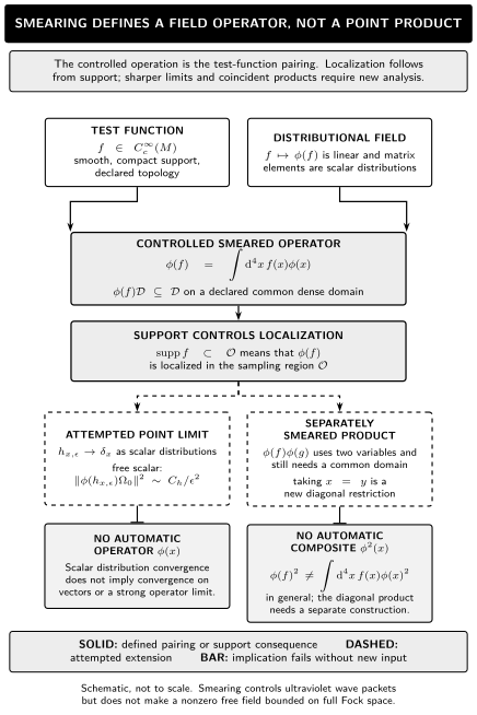
Smearing turns the field kernel into a controlled operator and support supplies localization, but neither a sharp-point operator nor a coincident product follows automatically. Dashed branches are attempted extensions and bars mark the missing implication; the free-scalar scaling shown for the point attempt is quantitative in its stated regime, while the map geometry is schematic and not to scale.

Read without the graphic: $f\mapsto\phi(f)$ is the defined linear pairing on a declared common domain, and $\operatorname{supp}f\subset\mathcal O$ supplies its localization region. Distributional convergence $h_{x,\epsilon}\to\delta_x$ does not imply a strong operator limit, while the two-variable product $\phi(f)\phi(g)$ does not by itself define the diagonal composite $\phi^2(x)$. Each extension requires new domain and ultraviolet input.

Distributional calculus

The familiar calculus of fields survives, but every identity is tested against smooth functions. The derivative of a field is defined by integration by parts:

$$(\partial_\mu\phi)(f) := -\phi(\partial_\mu f).$$

There is no boundary term because $f$ has compact support. Two derivatives reverse the sign twice, so the free Klein–Gordon equation

$$(\Box+m^2)\phi=0$$

means

$$\phi\!\left((\Box+m^2)f\right)=0.$$

This holds for every $f\in C_c^\infty(M)$.

Likewise, define the Pauli–Jordan distribution $\Delta$ by the convention

$$[\phi(x),\phi(y)] = i\Delta(x-y)\mathbf 1.$$

The actual operator statement is the smeared identity

$$\begin{aligned} [\phi(f),\phi(g)] &= i\Delta(f,g)\mathbf 1,\\ \Delta(f,g) &:= \int\mathrm d^4x\,\mathrm d^4y\\ &\quad\times f(x)\Delta(x-y)g(y). \end{aligned}$$

The causal support of $\Delta$ then implies $\Delta(f,g)=0$ when the two supports are spacelike separated. This is the scalar distributional check; graded locality and the distinction between fields and observables are developed on the later spacelike-compatibility page.

Hollands and Wald construct the advanced and retarded kernels and impose the field equation and commutator directly on smeared generators in Hollands and Wald 2015, arXiv v2, § 2.1, pp. 10–12. Their metric convention gives $(\Box_g-m^2)\phi=0$. Reversing the metric sign produces the site convention $(\Box+m^2)\phi=0$; the sign of $\Delta$ here is fixed by

$$[\phi(t,\mathbf x),\partial_0\phi(t,\mathbf y)] = i\delta^{(3)}(\mathbf x-\mathbf y)$$

as a spatially smeared identity.

First application: the free scalar field

Use the delta-normalized creators from the preceding particle pages,

$$\begin{aligned} [a(\mathbf p),a^\dagger(\mathbf q)] &= (2\pi)^3\delta^{(3)}(\mathbf p-\mathbf q),\\ a(\mathbf p)\Omega_0&=0, \qquad E_{\mathbf p}=\sqrt{\mathbf p^2+m^2}. \end{aligned}$$

With $p^0=E_{\mathbf p}$ and $p\cdot x=p^0x^0-\mathbf p\cdot\mathbf x$, the formal point-field expansion is

$$\begin{aligned} \phi(x) &= \int \frac{\mathrm d^3\mathbf p} {(2\pi)^3\sqrt{2E_{\mathbf p}}}\\ &\quad\times \left[ a(\mathbf p)e^{-ip\cdot x} + a^\dagger(\mathbf p)e^{ip\cdot x} \right]. \end{aligned}$$

Now declare the Fourier convention

$$\widetilde f(p) := \int\mathrm d^4x\, e^{ip\cdot x}f(x).$$

Only after smearing does the mode expansion define an operator on its working domain:

$$\begin{aligned} \phi(f) &= \int \frac{\mathrm d^3\mathbf p} {(2\pi)^3\sqrt{2E_{\mathbf p}}}\\ &\quad\times \left[ a(\mathbf p)\widetilde f(-p) + a^\dagger(\mathbf p)\widetilde f(p) \right]. \end{aligned}$$

The signs are forced by the Fourier convention: the annihilation wave $e^{-ip\cdot x}$ pairs with $\widetilde f(-p)$, while the creation wave pairs with $\widetilde f(p)$. For real $f$, these two coefficients are complex conjugates on the two mass shells.

Acting on the vacuum removes the annihilation part. With

$$\begin{aligned} \mathrm d\Pi_{\mathbf p} &= \frac{\mathrm d^3\mathbf p} {(2\pi)^3\,2E_{\mathbf p}},\\ |\mathbf p\rangle &= \sqrt{2E_{\mathbf p}}\, a^\dagger(\mathbf p)\Omega_0, \end{aligned}$$

one obtains

$$\begin{aligned} \phi(f)\Omega_0 &= \int\mathrm d\Pi_{\mathbf p}\, \widetilde f(p)|\mathbf p\rangle,\\ \left\|\phi(f)\Omega_0\right\|^2 &= \int\mathrm d\Pi_{\mathbf p}\, \left|\widetilde f(p)\right|^2. \end{aligned}$$

The last integral is finite for $f\in C_c^\infty$ because its Fourier transform decreases faster than any inverse power along the real mass shell. Thus a spacetime sampler creates a normalizable one-particle packet even though neither $a^\dagger(\mathbf p)$ nor $\phi(x)$ is a sharp-label Hilbert-space operator.

There is also a natural common domain in this free representation. Let $\mathscr D_{\mathrm{fin}}$ be the algebraic finite-particle subspace of bosonic Fock space. For a one-particle packet $h$ and an $n$-particle vector $\Psi_n$,

$$\begin{aligned} \|a(h)\Psi_n\| &\leq \sqrt n\,\|h\|\,\|\Psi_n\|,\\ \|a^\dagger(h)\Psi_n\| &\leq \sqrt{n+1}\,\|h\|\,\|\Psi_n\|. \end{aligned}$$

The on-shell restrictions of $\widetilde f$ supply the required square-integrable packets, so $\phi(f)$ maps $\mathscr D_{\mathrm{fin}}$ into itself. If the creation packet $h_f$ is nonzero, take normalized $n$-particle vectors with every slot occupied by $\widehat h_f=h_f/\|h_f\|$. Then

$$\left\| a^\dagger(h_f) \widehat h_f^{\otimes_s n} \right\| = \sqrt{n+1}\,\|h_f\|.$$

The creation and annihilation parts land in orthogonal particle-number sectors, so they cannot cancel this growth. Thus a smeared field with a nonzero creation packet is unbounded on the full Fock space. A smearing whose on-shell restriction vanishes instead represents the zero field, as the distributional Klein–Gordon equation requires.

Srednicki 2006, § 3, pp. 38–42 supplies the classical mode expansion, invariant mass-shell measure, and canonical commutators used here. Srednicki uses signature $(-+++)$ and creators normalized by

$$[a_{\mathrm S}(\mathbf p),a_{\mathrm S}^\dagger(\mathbf q)] = (2\pi)^3\,2E_{\mathbf p}\, \delta^{(3)}(\mathbf p-\mathbf q).$$

The conversion $a_{\mathrm S}(\mathbf p)=\sqrt{2E_{\mathbf p}}\,a(\mathbf p)$, together with the metric-sign reversal, gives exactly the site formulas above. The mass shell, vacuum norm, and equal-time bracket are unchanged.

A regulated attempt to reach a point

Smearing is not merely a formal change of notation. Let $h\in C_c^\infty(\mathbb R^4)$ be real with

$$\int\mathrm d^4y\,h(y)=1,$$

and concentrate it near $x_0$:

$$h_{x_0,\epsilon}(x) := \epsilon^{-4} h\!\left(\frac{x-x_0}{\epsilon}\right), \qquad \epsilon>0.$$

Then $h_{x_0,\epsilon}\to\delta_{x_0}$ as scalar distributions, and

$$\widetilde h_{x_0,\epsilon}(p) = e^{ip\cdot x_0}\widetilde h(\epsilon p).$$

Every regulated field $\phi(h_{x_0,\epsilon})$ is defined on $\mathscr D_{\mathrm{fin}}$. Nevertheless,

$$\left\| \phi(h_{x_0,\epsilon})\Omega_0 \right\|^2 = \int\mathrm d\Pi_{\mathbf p}\, \left|\widetilde h(\epsilon p)\right|^2.$$

Set $\mathbf k=\epsilon\mathbf p$ and define

$$\omega_{\epsilon,\mathbf k} := \sqrt{\mathbf k^2+\epsilon^2m^2}.$$

In four spacetime dimensions the norm becomes

$$\begin{aligned} \left\| \phi(h_{x_0,\epsilon})\Omega_0 \right\|^2 &= \frac{I_\epsilon}{\epsilon^2},\\ I_\epsilon &:= \int \frac{\mathrm d^3\mathbf k}{(2\pi)^3} \frac{ \left| \widetilde h\!\left( \omega_{\epsilon,\mathbf k}, \mathbf k \right) \right|^2 }{ 2\omega_{\epsilon,\mathbf k} }. \end{aligned}$$

Because $\widetilde h(0)=1$, the integral tends to a finite positive constant,

$$C_h = \int \frac{\mathrm d^3\mathbf k}{(2\pi)^3\,2|\mathbf k|} \left| \widetilde h(|\mathbf k|,\mathbf k) \right|^2 >0.$$

Consequently,

$$\left\| \phi(h_{x_0,\epsilon})\Omega_0 \right\|^2 \sim \frac{C_h}{\epsilon^2}.$$

The sampler converges to a delta distribution, but the sampled field does not converge strongly on the vacuum. A distributional limit of test functions therefore does not imply an operator limit. This explicit free-field calculation is the ultraviolet obstruction hidden by the symbol $\phi(x)$.

Smearing and multiplication are different operations

Separate smearing in two variables can make a bilocal product meaningful:

$$\begin{aligned} \phi(f)\phi(g) &\ \sim\ \int\mathrm d^4x\,\mathrm d^4y\, \\ &\quad\times f(x)g(y)\phi(x)\phi(y), \end{aligned}$$

where the right-hand side is only kernel notation and a common operator domain is still required. This is not a definition of a coincident composite field. In particular,

$$\phi(f)^2 \neq \int\mathrm d^4x\,f(x)\phi(x)^2$$

in general: the left side smears two independent variables with $f(x)f(y)$ before multiplying, whereas the right side tries to restrict a singular two-point distribution to the diagonal $x=y$.

Similarly, a state can assign a well-defined distribution

$$W_2(f,g) := \langle\Omega,\phi(f)\phi(g)\Omega\rangle$$

without making $W_2(x,x)$ meaningful. Ordinary pointwise multiplication of distributions is not automatic, so a composite such as $\phi^2$ needs a separate construction. This limitation is emphasized in Hollands and Wald 2015, arXiv v2, § 1, p. 5. Wick products, point splitting, contact terms, and interacting composite-operator renormalization are developed later rather than being smuggled into the notation here.

What remains meaningful before axioms

The following statements require no fictional point operator:

• linearity and test-function continuity of $f\mapsto\phi(f)$;
• support and localization statements formulated through $\operatorname{supp}f$;
• distributional derivatives, field equations, and causal commutators;
• matrix elements and $n$-point functions as scalar distributions;
• products of separately smeared fields when an abstract algebra or common invariant domain has been specified; and
• regulated point approximations with an explicit topology and a check of whether an operator, vector, or distributional limit exists.

What this physics-first formulation does not settle is equally important. It does not select a maximal operator domain, prove closability or self-adjointness, impose the spectrum condition, state a microlocal regularity condition, reconstruct a Hilbert space, or turn pointlike fields into a net of local algebras.

For the test-function foundations, see Test-Function Spaces, Distributions, Support, and Convergence, Convolution, Approximate Identities, and Poisson Summation, and Locally Convex, Nuclear, and Rigged Hilbert Spaces. The theorem-first domain and axiom treatment belongs to Wightman Fields, Domains, and Axioms; the passage from fields to local algebras belongs to From Pointlike Fields to Nets and Affiliated Operators.

Within this chapter, continue to Fields, Observables, and Interpolating Operators for the field-versus-observable distinction and to Spacelike Compatibility and Local Observables for graded locality. Coincident products are treated in Local and Composite Operator Insertions, Free Wick Products and Point Splitting, and Coincident Products and Contact Terms.

Common pitfalls

“A distribution is just a badly behaved function.” A distribution is a continuous linear functional on a declared test-function space. It need not possess point values at all.

“Smearing makes the field a bounded operator.” In the free theory $\phi(f)$ is well defined on the finite-particle domain, but for a nonzero on-shell packet its action on suitable $n$-particle vectors grows at least like $\sqrt n$. Smearing controls the momentum packet, not the particle-number growth.

“An approximate identity defines $\phi(x)$ by a limit.” The functions $h_{x,\epsilon}$ converge to $\delta_x$ only in the scalar distribution topology. The free-field vacuum norm grows as $\epsilon^{-1}$, so the corresponding operators have no strong point limit on a domain containing the vacuum.

“If $\phi(f)$ exists, then $\phi^2(f)$ exists.” Smearing a linear field and defining a coincident product are separate problems. The latter requires new information about singular products and their extension to the diagonal.

Check your understanding

1. Starting from the formal free-field expansion and the stated Fourier convention, derive the two arguments $\widetilde f(-p)$ and $\widetilde f(p)$ in $\phi(f)$.

   Answer

   The annihilation term contains $e^{-ip\cdot x}$, so its spacetime integral is $\int\mathrm d^4x\,f(x)e^{-ip\cdot x}=\widetilde f(-p)$. The creation term contains $e^{ip\cdot x}$ and therefore gives $\widetilde f(p)$. For real $f$, Fourier conjugation gives $\widetilde f(-p)=\overline{\widetilde f(p)}$.

2. Why does $h_{x,\epsilon}\to\delta_x$ fail to define a point field even though every $\phi(h_{x,\epsilon})$ is defined?

   Answer

   Distributional convergence tests $h_{x,\epsilon}$ against smooth scalar functions. An operator limit is stronger and must be checked on vectors in a common domain. For the free vacuum, the norm squared of $\phi(h_{x,\epsilon})\Omega_0$ grows as $\epsilon^{-2}$, so the vectors cannot converge in Hilbert-space norm and the operators cannot converge strongly on the vacuum.

References

• Hollands, Stefan, and Robert M. Wald. “Quantum Fields in Curved Spacetime.” Physics Reports 574 (2015): 1–35. DOI. Open PDF, arXiv:1401.2026v2.
• Srednicki, Mark. Quantum Field Theory. Author-hosted manuscript, University of California, Santa Barbara, 2006. Author’s manuscript page.