

The Action Principle and Field Equations
Stationary action turns a local density into differential equations only after the allowed variations and their boundary behavior have been specified. For a first-derivative action, one integration by parts separates the first variation into a bulk Euler–Lagrange term and a surface term. Vanishing of the bulk term for every compactly supported variation gives the local field equations; it does not by itself choose boundary conditions, prove that solutions exist, or make the stationary configuration a minimum.
This page derives that statement on a finite spacetime region and applies it to a real scalar field and the Maxwell potential. The design of boundary data and boundary functionals belongs to the next page; higher-derivative stability, PDE well-posedness, Hamiltonian constraints, and path-integral quantization are outside the present scope.
Helpful background. Fields, Configurations, Dimensions, and Local Dynamics distinguishes raw configurations, on-shell fields, and solutions of a posed problem. Field Variations and Boundary Terms develops the reusable variational calculus.
Stationarity for a local field action
Section titled “Stationarity for a local field action”Let be a spacetime region with sufficiently regular boundary, and let denote a collection of real field components. Consider
A variation is a one-parameter family of admissible configurations
where has the same tensor type and reality properties as . The first variation is the directional derivative on configuration space,
This is not a spacetime derivative. It compares nearby configurations while holding the spacetime point fixed. For complex fields one may instead vary the real and imaginary parts, or vary a declared pair of independent variables; the choice must be stated before differentiating.
The action is stationary at relative to a chosen class of variations when for every allowed . Stationary does not mean smallest: the second variation may have positive, negative, or null directions. The field-theoretic action principle and its local equations are developed in Schwartz 2014, §§ 3.1–3.2, pp. 29–32 and Weinberg 1995, § 7.2, pp. 300–305.
The bulk–boundary split
Section titled “The bulk–boundary split”Assume that differentiation with respect to may be passed through the integral and that the fields are regular enough for the product rule and divergence theorem. Direct differentiation gives
Define the derivative momentum and Euler–Lagrange expression by
The product rule,
then yields the central decomposition
The figure makes the logical fork explicit. Follow the solid branch when compact support is used to isolate the interior equation; follow the dashed branch when boundary variations remain and the chosen boundary-data space must be tested.
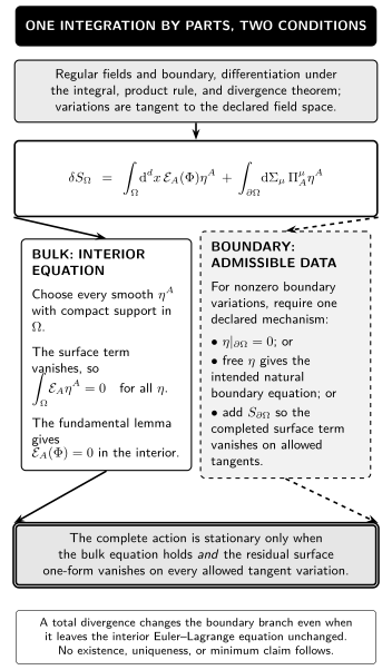
For a regular first-derivative action on a finite region, one integration by parts produces a bulk term and a surface one-form. Compactly supported variations test only the interior Euler–Lagrange equation; stationarity of the complete action additionally requires the residual surface one-form to vanish on every allowed boundary tangent variation. The diagram is schematic and does not assert a minimum or analytic PDE well-posedness.
| Part of the variation | Allowed variations or added data | Consequence of stationarity |
|---|---|---|
| Bulk term | Every smooth compactly supported | in the interior by the fundamental lemma |
| Original surface term | Dirichlet tangent variations with at the boundary | The original surface term vanishes on the allowed variation space |
| Original surface term with free boundary variation | Boundary values are allowed to vary | The coefficient of each free variation supplies the intended natural boundary equation |
| Completed surface term | Add and test the original surface term plus on the declared tangent variations | The residual surface one-form must vanish; the chosen boundary variable and action are matched |
Here is the outward-directed surface element. If has compact support in the interior of , the surface integral vanishes. Stationarity then implies
for every smooth compactly supported . The fundamental lemma of the calculus of variations gives the Euler–Lagrange equations
The quantifier “for every allowed variation” matters. If a field obeys an algebraic constraint, the variations must be tangent to that constraint. If a gauge symmetry makes some variations redundant, the resulting Euler–Lagrange expressions satisfy identities; stationarity does not automatically fix a gauge.
Compact support is a clean way to derive the interior equations, but it deliberately avoids the boundary problem. With nonzero boundary variations, one must instead choose boundary data or add a boundary functional so that the complete surface variation vanishes. This action-plus-boundary-data formulation is explained in Harlow and Wu 2020, § 2.2, pp. 9–12 and developed here on Boundaries, Variations, and Well-Posed Actions.
A related qualification concerns total divergences. If
then
The two densities give the same interior Euler–Lagrange equations under compactly supported variations, but they need not define the same boundary variational problem. “Drop the total derivative” is therefore a conditional operation, not an algebraic identity between actions on arbitrary regions. The integration-by-parts step is displayed in Schwartz 2014, § 3.2, pp. 31–32, while its boundary-sensitive formulation is given in Harlow and Wu 2020, § 2.2, pp. 9–12.
The scalar field: Klein–Gordon from stationarity
Section titled “The scalar field: Klein–Gordon from stationarity”For a real scalar with potential , take
Under ,
where . For compactly supported , stationarity gives
For , this becomes the Klein–Gordon equation
This derivation and sign choice are checked in Schwartz 2014, § 3.2, pp. 31–32. The surface term also shows what compact support hid: fixing to vanish at the boundary removes it, while allowing arbitrary boundary values would require a different condition or a compensating boundary term. The scalar example is worked boundary-sensitively in Harlow and Wu 2020, § 3.2, p. 21.
The equation is a local differential condition on an on-shell configuration. It is not yet a solution: one must still specify compatible initial or boundary data and establish the relevant existence and uniqueness result. The mode structure of the free equation is developed on The Klein–Gordon Field and Its Modes.
Maxwell dynamics and the kinematic identity
Section titled “Maxwell dynamics and the kinematic identity”For a real Maxwell potential, let
Write the variation as . Then
Antisymmetry of combines the two terms in , so
Compactly supported variations therefore give the vacuum Maxwell equations
The other familiar relation,
is not a second Euler–Lagrange equation. It follows identically from and commutativity of partial derivatives. The Maxwell action and its field equations are presented in Schwartz 2014, § 8.2.3, pp. 118–119.
Two checks expose the gauge structure without completing its constraint analysis. First, a gauge-direction variation gives , so the action is stationary in that direction even away from a solution. Second,
holds identically by antisymmetry. This identity relates the component Euler–Lagrange expressions; it neither imposes nor counts physical polarizations. Those questions belong to The Free Maxwell Field and Gauge Redundancy. If is nonzero at , the remaining surface term must also be analyzed rather than silently discarded.
What the derivation proves—and does not
Section titled “What the derivation proves—and does not”The argument proves a conditional implication:
Its hypotheses carry the real content: the action must be differentiable on the declared field space, integrations by parts must be legitimate, and the test variations must be rich enough for the fundamental lemma. For fields with constrained target spaces, corners, singularities, nonlocal terms, or higher derivatives, this simple formula must be modified or applied with additional care.
The converse is also boundary-sensitive. A field satisfying the bulk equations makes the bulk part of vanish, but the complete action is stationary only if the remaining surface variation vanishes for the allowed data. Nor does either statement establish a well-posed PDE problem. The next two chapter pages separate these questions: Boundaries, Variations, and Well-Posed Actions treats differentiability at the boundary, while Hamiltonian Initial Data and Phase Space reorganizes the dynamics as initial-value evolution.
Common pitfalls
Section titled “Common pitfalls”“Least action” does not guarantee a minimum. The first variation tests stationarity. Stability requires information from the second variation, the Hamiltonian, and the allowed perturbations.
A total derivative is not simply zero. It becomes a boundary integral. It may be harmless for compact support or specified falloff, but it can change boundary conditions, charges, and the differentiability of the action.
A gauge variation is not a gauge choice. The Maxwell action is invariant along . That degeneracy does not impose Lorenz or Coulomb gauge.
The Bianchi identity is not the Maxwell equation. follows from the definition of . The equation follows from stationary action.
An equation is not a solved problem. Euler–Lagrange equations identify on-shell configurations locally. Initial or boundary data, regularity, existence, uniqueness, and gauge reduction remain separate tasks.
Check your understanding
Section titled “Check your understanding”-
Add a source term to the scalar density and derive the field equation.
Solution
The source contributes to the first variation. The bulk coefficient becomes , so stationarity gives
The kinetic surface term is unchanged.
-
Show directly that replacing by leaves the interior Euler–Lagrange equations unchanged for compactly supported variations.
Solution
The action changes by . Its variation is also supported on , so it vanishes when has compact support in the interior. Therefore the bulk coefficient multiplying arbitrary interior is unchanged. This does not assert equivalence for nonzero boundary variations.
-
Insert into the Maxwell variation before integrating by parts.
Solution
Commutativity of partial derivatives gives
Hence identically along the gauge direction. This is an off-shell invariance, not the dynamical equation .
The action principle has now done exactly one job: it converted a differentiable local action and a declared class of variations into bulk field equations plus an explicit surface term. The next page asks what must happen to that surface term when the boundary cannot be ignored.
References
Section titled “References”- Harlow, Daniel, and Jie-qiang Wu. “Covariant Phase Space with Boundaries.” Journal of High Energy Physics 2020, no. 10 (2020): 146. DOI.
- Schwartz, Matthew D. Quantum Field Theory and the Standard Model. Cambridge: Cambridge University Press, 2014. DOI.
- Weinberg, Steven. The Quantum Theory of Fields. Volume I: Foundations. Cambridge: Cambridge University Press, 1995. DOI.
Original QFT.org content:CC BY 4.0, unless an item supplies different terms. Third-party material retains its own terms.