Time Slicing and Transition Amplitudes

For a fixed spatial regulator with finitely many real field coordinates, time slicing rewrites a transition amplitude as a sequence of finite-dimensional configuration and momentum integrals. In Lorentzian signature these are oscillatory boundary values, not probability integrals. Coordinate resolutions of the identity expose the intermediate configurations, momentum resolutions produce a phase-space exponent, and a declared short-time ordering rule determines where each coordinate is sampled. If the momentum dependence is a nonsingular quadratic form, every momentum integral can then be performed exactly, including its normalization and oscillatory branch.

Three steps must remain distinct. Inserting identities is exact; replacing each short evolution factor by a chosen symbol or operator splitting is an approximation or regulator; and taking the number of slices to infinity is a further limit. Endpoint wave functions determine which states are prepared, while removal of the spatial regulator is yet another problem. This page derives those statements for a finite bosonic system and applies them to the regulated free scalar. It does not construct a continuum Lorentzian measure or treat constrained gauge systems.

Required background. Regulated Bosonic Field Integrals supplies the finite-coordinate regulator and the distinction between a defined integral and formal continuum notation. Schrödinger Wave Functionals supplies configuration eigenstates, finite-mode Hamiltonians, and the boundary wave functions used below.

Helpful background. Canonical Quantization: Algebra, Representation, and State supplies the regulated canonical relations and explains why the algebra, its representation, and the chosen state are separate data.

Identity insertions turn finite evolution into a multiple integral

Fix a spatial regulator that leaves $M<\infty$ independent real coordinates. In the Schrödinger representation, use generalized configuration and momentum bases normalized by

$$\begin{aligned} \langle \mathbf q'|\mathbf q\rangle &=\delta^{(M)}(\mathbf q'-\mathbf q), & \int_{\mathbb R^M}\mathrm d^M q\, |\mathbf q\rangle\langle\mathbf q| &=\mathbf 1, \\ \langle\mathbf q|\mathbf p\rangle &=(2\pi)^{-M/2}e^{i\mathbf p\cdot\mathbf q}, & \int_{\mathbb R^M}\mathrm d^M p\, |\mathbf p\rangle\langle\mathbf p| &=\mathbf 1 . \end{aligned}$$

Let the time-independent Hamiltonian $\widehat H_\Lambda$ be self-adjoint on the regulated Hilbert space, let $T=t_f-t_i>0$, and set

$$\Delta t=\frac{T}{N}, \qquad \mathbf q_0=\mathbf q_i, \qquad \mathbf q_N=\mathbf q_f.$$

The fixed-endpoint kernel is

$$K_\Lambda(\mathbf q_f,T;\mathbf q_i,0) = \langle\mathbf q_f| e^{-i\widehat H_\Lambda T} |\mathbf q_i\rangle .$$

Because $e^{-i\widehat H_\Lambda T} =[e^{-i\widehat H_\Lambda\Delta t}]^N$, inserting $N-1$ coordinate identities gives the exact relation

$$\begin{aligned} K_\Lambda(\mathbf q_f,T;\mathbf q_i,0) ={}& \int_{\mathbb R^{M(N-1)}} \prod_{r=1}^{N-1}\mathrm d^M q_r \\ &\times \prod_{r=0}^{N-1} \langle\mathbf q_{r+1}| e^{-i\widehat H_\Lambda\Delta t} |\mathbf q_r\rangle . \end{aligned}$$

There are exactly $N$ short evolution factors but only $N-1$ internal configuration integrations; the endpoints remain fixed. Nothing in this identity has yet replaced an operator by an action, introduced a momentum integral, or taken a limit. The same composition step underlies the standard quantum-mechanical and field-theoretic constructions in Schwartz 2014, § 14.2, pp. 254–260 and Weinberg 1995, § 9.1, pp. 378–384.

For a time-dependent Hamiltonian, the factors carry their own slice times and their order matters. The rest of this page keeps $\widehat H_\Lambda$ time independent so that the role of operator ordering inside one slice is not confused with chronological ordering of different slices.

Momentum insertions produce the phase-space action

A particularly transparent slicing prescription applies when

$$\widehat H_\Lambda = \mathcal T(\widehat{\mathbf p})+V(\widehat{\mathbf q}).$$

Define the left-endpoint product

$$U_N(T) = \left[ e^{-i\Delta t\,\mathcal T(\widehat{\mathbf p})} e^{-i\Delta t\,V(\widehat{\mathbf q})} \right]^N .$$

This equation defines a concrete regulated evolution operator for every finite $N$. Since the rightmost factor acts first, one momentum identity in a single interval gives

$$\begin{aligned} &\langle\mathbf q_{r+1}| e^{-i\Delta t\,\mathcal T(\widehat{\mathbf p})} e^{-i\Delta t\,V(\widehat{\mathbf q})} |\mathbf q_r\rangle \\ &\quad = \int_{\mathbb R^M}\frac{\mathrm d^M p_r}{(2\pi)^M} \exp\!\left\{ i\left[ \mathbf p_r\cdot(\mathbf q_{r+1}-\mathbf q_r) -\Delta t\, \bigl(\mathcal T(\mathbf p_r)+V(\mathbf q_r)\bigr) \right] \right\}. \end{aligned}$$

Consequently the kernel of $U_N(T)$ is exactly the finite multiple integral

$$\begin{aligned} K_{\Lambda,N}^{\mathrm{ps}} ={}& \int \prod_{r=1}^{N-1}\mathrm d^M q_r \prod_{r=0}^{N-1} \frac{\mathrm d^M p_r}{(2\pi)^M} \\ &\times \exp\!\left\{ i\sum_{r=0}^{N-1} \left[ \mathbf p_r\cdot\Delta\mathbf q_r -\Delta t\, \bigl(\mathcal T(\mathbf p_r)+V(\mathbf q_r)\bigr) \right] \right\}, \end{aligned}$$

where $\Delta\mathbf q_r=\mathbf q_{r+1}-\mathbf q_r$. Thus one obtains $N$ momentum integrations, one for each interval. The expression is finite-dimensional, but it is oscillatory rather than an integral against a probability measure.

The target evolution is recovered only if the product has an appropriate limit,

$$\underset{N\to\infty}{\operatorname{s\!-\!lim}}\, U_N(T) =e^{-i\widehat H_\Lambda T},$$

where the equality is a strong-operator statement under suitable product-formula and domain hypotheses. For unbounded Schrödinger operators, this statement is not licensed by a pointwise Taylor expansion alone, and an operator limit need not imply pointwise convergence of every kernel. The finite formula above remains useful because its object and approximation are explicit.

Ordering lives inside each time slice

For a general Hamiltonian containing noncommuting coordinates and momenta, a classical-looking function $H(\mathbf p,\mathbf q)$ does not determine a unique operator. Conversely, an operator ordering determines how its short-step symbol samples a slice:

Declared operator or splitting	Coordinate sampled in the short-step symbol	What must remain visible
$e^{-i\Delta t \mathcal T(\widehat p)}e^{-i\Delta t V(\widehat q)}$	Initial endpoint $\mathbf q_r$	Left-endpoint rule used above
$e^{-i\Delta t V(\widehat q)}e^{-i\Delta t \mathcal T(\widehat p)}$	Final endpoint $\mathbf q_{r+1}$	Reversed split, not the same finite-$N$ kernel
All $\widehat q$‘s to the left of all $\widehat p$‘s	Final endpoint in the corresponding short-step matrix element	The ordering convention behind the symbol
All $\widehat p$‘s to the left of all $\widehat q$‘s	Initial endpoint	The opposite convention
Weyl-symmetric ordering	Midpoint to leading short-time order	The Weyl symbol and its accuracy

For bounded operators, the Baker–Campbell–Hausdorff expansion displays the leading split error:

$$\begin{aligned} e^{-i\Delta t\widehat{\mathcal T}} e^{-i\Delta t\widehat V} = \exp\!\left[ -i\Delta t(\widehat{\mathcal T}+\widehat V) -\frac{\Delta t^2}{2} [\widehat{\mathcal T},\widehat V] +O(\Delta t^3) \right]. \end{aligned}$$

The local error is then $O(\Delta t^2)$, giving the familiar $O(T\Delta t)$ accumulated scale when a norm estimate is valid. The symmetric split

$$e^{-i\Delta t\widehat V/2} e^{-i\Delta t\widehat{\mathcal T}} e^{-i\Delta t\widehat V/2}$$

cancels the leading commutator term and has local $O(\Delta t^3)$ error under the corresponding regularity assumptions. These error orders are not automatic for unbounded operators; common invariant domains and suitable commutator control are part of the claim.

Endpoint and midpoint rules may converge to the same simple $\mathcal T(\widehat p)+V(\widehat q)$ Hamiltonian, but they cannot be interchanged silently. For field-dependent kinetic terms, the determinant generated by momentum elimination is itself configuration dependent, so changing the discretization without matching the operator ordering changes the finite prescription. Weinberg derives the connection between the discretized measure and operator order, warns that another interpretation of the measure gives another prescription, and exhibits the field-dependent determinant Weinberg 1995, §§ 9.1 and 9.3, p. 384 and pp. 389–394.

Quadratic momenta give the configuration-space factor

Assume now that the slice Hamiltonian has constant, positive quadratic momentum dependence,

$$H(\mathbf p,\mathbf q) = \frac12 \mathbf p^{\mathsf T}A^{-1}\mathbf p +V(\mathbf q), \qquad A=A^{\mathsf T}>0.$$

The Lorentzian momentum integral needs a branch prescription. Introduce Gaussian damping and take its boundary value:

$$\begin{aligned} G_{\varepsilon}(\Delta\mathbf q) ={}& \int_{\mathbb R^M} \frac{\mathrm d^M p}{(2\pi)^M} \\ &\times \exp\!\left[ i\mathbf p\cdot\Delta\mathbf q -\frac{\varepsilon+i\Delta t}{2} \mathbf p^{\mathsf T}A^{-1}\mathbf p \right], \qquad \varepsilon>0 . \end{aligned}$$

Completing the square gives

$$\lim_{\varepsilon\downarrow0} G_\varepsilon(\Delta\mathbf q) = \frac{(\det A)^{1/2}} {(2\pi i\Delta t)^{M/2}} \exp\!\left[ \frac{i}{2\Delta t} \Delta\mathbf q^{\mathsf T} A\Delta\mathbf q \right],$$

with the square-root branch reached continuously from $\varepsilon>0$. Performing all $N$ momentum integrations therefore yields

$$\begin{aligned} K_{\Lambda,N}^{\mathrm{conf}} ={}& \frac{(\det A)^{N/2}} {(2\pi i\Delta t)^{MN/2}} \int \prod_{r=1}^{N-1}\mathrm d^M q_r\, e^{iS_{\Lambda,N}}, \\ S_{\Lambda,N} ={}& \sum_{r=0}^{N-1} \left[ \frac{ \Delta\mathbf q_r^{\mathsf T} A\Delta\mathbf q_r }{2\Delta t} -\Delta t\,V(\mathbf q_r) \right]. \end{aligned}$$

The prefactor is part of the kernel. Its power is fixed by $N$ momentum integrations, and together with the $N-1$ configuration measures it leaves the final kernel with the units of $\delta^{(M)}(\mathbf q_f-\mathbf q_i)$.

The Euclidean short step can be derived independently from $e^{-\Delta\tau\widehat H_\Lambda}$ rather than inferred from a bare substitution:

$$\begin{aligned} &\langle\mathbf q_{r+1}| e^{-\Delta\tau\mathcal T(\widehat{\mathbf p})} e^{-\Delta\tau V(\widehat{\mathbf q})} |\mathbf q_r\rangle \\ &\quad = \frac{(\det A)^{1/2}} {(2\pi\Delta\tau)^{M/2}} \exp\!\left[ -\frac{ \Delta\mathbf q_r^{\mathsf T} A\Delta\mathbf q_r }{2\Delta\tau} -\Delta\tau V(\mathbf q_r) \right]. \end{aligned}$$

This is a decaying Gaussian when the potential is stable. Its relation to a Lorentzian amplitude still requires analytic, contour, and state data.

The Gaussian elimination is not a universal Legendre transform. A coordinate-dependent $A(\mathbf q)$ produces slice-dependent determinants and ordering questions; a singular quadratic form signals constraints or zero directions; and a nonquadratic momentum dependence is not removed by this Gaussian calculation. The precise quadratic hypothesis and its determinant qualifications are developed in Weinberg 1995, § 9.3, pp. 389–394.

The sequence of exact identities, ordering-dependent short steps, Gaussian reduction, and the separate slicing limit is summarized below.

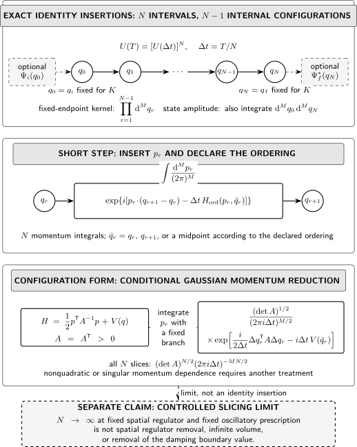
Schematic finite time slicing, not to scale. For a fixed-endpoint kernel, the top panel has $N$ intervals and $N-1$ internal configuration integrations. When the dashed endpoint wave functions are attached to form a state-to-state amplitude, $q_0$ and $q_N$ are also integrated, each exactly once. The middle panel adds $N$ momentum integrations and a declared coordinate-sampling rule. The third panel integrates momenta only for a nonsingular positive quadratic form and retains the determinant, slice normalization, and oscillatory branch. The dashed final arrow is the controlled $N\to\infty$ limit at fixed spatial regulator; it does not remove that regulator, take infinite volume, or erase the boundary-value prescription.

Read the diagram from top to bottom: the solid first row is a completeness identity; the phase-space row represents the chosen short-step prescription; the horizontal Gaussian arrow is exact only under its displayed quadratic hypothesis; and the dashed downward arrow is a limit claim. Open the SVG alone for scalable zoom and pan.

Composition and the short-time delta fix normalization

The exact evolution kernel satisfies

$$\begin{aligned} K_\Lambda( \mathbf q_f,T_1+T_2; \mathbf q_i,0) = \int_{\mathbb R^M}\mathrm d^M q\, K_\Lambda( \mathbf q_f,T_2; \mathbf q,0) K_\Lambda( \mathbf q,T_1; \mathbf q_i,0). \end{aligned}$$

It also has the distributional initial condition

$$\lim_{T\downarrow0} K_\Lambda(\mathbf q_f,T;\mathbf q_i,0) = \delta^{(M)}(\mathbf q_f-\mathbf q_i).$$

These two relations are normalization tests, not optional conventions. For $V=0$, the one-interval Gaussian gives

$$\begin{aligned} K_{0,A}(\mathbf q_f,T;\mathbf q_i,0) = \frac{(\det A)^{1/2}} {(2\pi iT)^{M/2}} \exp\!\left[ \frac{i}{2T} (\mathbf q_f-\mathbf q_i)^{\mathsf T} A(\mathbf q_f-\mathbf q_i) \right]. \end{aligned}$$

A direct Gaussian convolution reproduces the same expression with $T=T_1+T_2$, and testing it against a smooth compactly supported function gives the delta initial condition. Dropping $(\det A)^{1/2}(2\pi iT)^{-M/2}$ destroys both checks. Dividing by a vacuum amplitude can cancel field-independent factors in normalized correlators, but it does not license deleting the normalization of a transition kernel whose endpoint composition is being asserted.

Free scalar modes supply the field-theory check

Apply the construction to a real scalar with a finite spatial regulator. In independent real-mode coordinates, its free Hamiltonian is

$$\widehat H_\Lambda = \frac12 \widehat{\mathbf p}^{\mathsf T} \widehat{\mathbf p} +\frac12 \widehat{\mathbf q}^{\mathsf T} \Omega_\Lambda^2 \widehat{\mathbf q},$$

where $\Omega_\Lambda^2$ is real symmetric and nonnegative. First take all $\omega_\alpha>0$; a zero mode is treated below by a continuous limit. Choose an orthogonal matrix $O$ such that

$$O^{\mathsf T}\Omega_\Lambda^2O = \operatorname{diag} (\omega_1^2,\ldots,\omega_M^2), \qquad \boldsymbol\xi=O^{\mathsf T}\mathbf q .$$

These $\mathbf q$ are canonically normalized real-mode amplitudes. If one instead uses unrescaled lattice-site fields in $s$ spatial dimensions, the kinetic matrix carries the cell-volume factor $a^s$; the slice determinant and kinetic phase must carry the same factor. A time lattice spacing $\Delta t$ must not be confused with the spatial spacing $a$.

The orthogonal change of variables preserves $\mathrm d^M q$, so the kernel factorizes into $M$ oscillator kernels:

$$K_\Lambda( \mathbf q_f,T; \mathbf q_i,0) = \prod_{\alpha=1}^{M} K_{\omega_\alpha} (\xi_{f,\alpha},T; \xi_{i,\alpha},0).$$

For one positive-frequency mode and away from caustic times, the result is

$$\begin{aligned} K_\omega(q_f,T;q_i,0) ={}& \lim_{\varepsilon\downarrow0} \left[ \frac{\omega} {2\pi i\sin\!\bigl(\omega(T-i\varepsilon)\bigr)} \right]^{1/2} \\ &\times \exp\!\left\{ \frac{i\omega}{ 2\sin\!\bigl(\omega(T-i\varepsilon)\bigr)} \left[ (q_f^2+q_i^2) \cos\!\bigl(\omega(T-i\varepsilon)\bigr) -2q_fq_i \right] \right\}. \end{aligned}$$

The square root is continued from small positive $T$. At $T=n\pi/\omega$, the displayed quotient is not an ordinary function; the boundary value and composition law give a delta distribution with the corresponding caustic phase. A discrete time-slicing derivation of both the extended kernel and its exact delta-supported values at the caustics is given in Funahashi 2010, §§ 1–2, Open PDF pp. 1–2 and 6–8. In the limit $\omega\to0$, the formula becomes the free-particle kernel, so a massless regulated zero mode is propagated as a free coordinate even though it does not possess the normalizable oscillator vacuum discussed on the wave-functional page.

This expression supplies three independent checks:

• expanding $\sin\omega T$ and $\cos\omega T$ for $T\downarrow0$ reproduces the free short-time Gaussian and hence the delta initial condition;
• differentiating with respect to $T$ gives $i\partial_TK_\omega =[-\tfrac12\partial_{q_f}^2+\tfrac12\omega^2q_f^2]K_\omega$;
• summing the oscillator energy eigenfunctions with factors $e^{-i\omega(n+1/2)(T-i\varepsilon)}$ gives the same kernel, independently of the sliced integral.

Thus the first field-theory application is exact at fixed spatial regulator: the free scalar transition kernel is the product of the kernels obtained by taking the slicing limit of its finitely many oscillator coordinates. This does not yet assert a continuum field kernel.

Boundary wave functions change the amplitude being computed

The fixed-endpoint kernel is not itself an amplitude between arbitrary states. If $\Psi_i$ and $\Psi_f$ are normalized Schrödinger wave functions on the regulated configuration space, then

$$\begin{aligned} \mathcal A_{fi}(T) ={}& \langle\Psi_f| e^{-i\widehat H_\Lambda T} |\Psi_i\rangle \\ ={}& \int\mathrm d^M q_f \int\mathrm d^M q_i\, \Psi_f^*(\mathbf q_f) K_\Lambda(\mathbf q_f,T;\mathbf q_i,0) \Psi_i(\mathbf q_i). \end{aligned}$$

The bulk Hamiltonian determines propagation, while the endpoint wave functions select the initial and final states. Replacing them by vacuum wave functions, integrating over a shared endpoint, or extending a contour changes the object being computed. Boundaries and State Preparation develops those operations, including vacuum projection and gluing; they are not consequences of writing $e^{iS}$ alone.

In particular, the $\varepsilon>0$ used above to choose the branch of a finite oscillatory momentum Gaussian does not by itself choose the Feynman vacuum. State selection comes from endpoint wave functions or an equivalent asymptotic boundary prescription.

The slicing limit is separate from other limits

Several operations are often compressed into one formal symbol even though they answer different questions:

Operation	Data held fixed	What a successful result establishes
$N\to\infty$	Spatial regulator, volume, Hamiltonian, endpoints, ordering sequence, and oscillatory prescription	The sliced operators or kernels approach the target regulated evolution
$\varepsilon\downarrow0$	Regulated Hamiltonian and endpoints	A specified Lorentzian boundary value or distribution
Spatial cutoff removal	Time prescription, observables, state, and tuning conditions	A continuum field-theory limit, if it exists
Infinite-volume limit	Ultraviolet regulator and local data	Removal of the infrared box, if controlled
Lorentzian–Euclidean continuation	Analytic domain, contour, state, and singularities	A relation between distinct boundary-value problems under stated hypotheses

Only the first operation is the time-slicing limit derived here. Even at fixed $M$, the Lorentzian integrand has unit modulus before damping and is not a probability density. Taking $N\to\infty$ therefore does not manufacture an ordinary measure on pointwise real-time paths. The evidence-supported conclusion is narrower: identity insertions and a controlled product limit represent a regulated transition kernel, with endpoints, normalization, ordering, and the oscillatory prescription retained.

Common pitfalls

Calling identity insertion a path integral derivation. Coordinate completeness gives an exact product of short kernels. An action appears only after a momentum insertion and a declared short-step symbol or splitting.

Dropping the per-slice factor. The powers of $2\pi$, $\Delta t$, and $\det A$ enforce the delta initial condition and composition. A normalization that cancels in a particular ratio may still be indispensable for the kernel itself.

Using midpoint and endpoint notation interchangeably. These rules encode operator ordering. Their differences are especially consequential for mixed coordinate–momentum products and coordinate-dependent kinetic terms.

Treating the Lorentzian weight as a probability measure. The finite integrals are oscillatory boundary values. Euclidean damping produces a different object whose relation to Lorentzian evolution requires analytic and state data.

Combining independent limits. Increasing the number of time slices does not remove a spatial cutoff, send the volume to infinity, or remove an $i0$ prescription.

Forgetting the boundary state. A bulk action with fixed endpoint fields defines a kernel. A vacuum amplitude, excited-state matrix element, or glued amplitude requires the corresponding endpoint wave functions and integrations.

Check your understanding

Use the worked solutions to compare each step with the normalization, ordering, and boundary data in the derivation.

1. For $N$ intervals, count the coordinate and momentum integrations in the phase-space slicing with fixed endpoints.

Answer

There are $N-1$ internal coordinate integrations, $\prod_{r=1}^{N-1}\mathrm d^M q_r$, because $\mathbf q_0$ and $\mathbf q_N$ are fixed. There are $N$ momentum integrations, one for every short evolution factor. The endpoints become two additional coordinate integrations only after boundary wave functions are attached to form a state-to-state amplitude.

2. Recover the determinant and $\Delta t$ powers in one quadratic momentum integral.

Answer

With $B=(\varepsilon+i\Delta t)A^{-1}$ and $\mathbf J=i\Delta\mathbf q$, the standard Gaussian formula gives

$$(2\pi)^{-M/2}(\det B)^{-1/2} \exp(\mathbf J^{\mathsf T}B^{-1}\mathbf J/2).$$

Since $(\det B)^{-1/2} =(\det A)^{1/2}(\varepsilon+i\Delta t)^{-M/2}$, the boundary value is $(\det A)^{1/2}(2\pi i\Delta t)^{-M/2}$ times the displayed kinetic phase. The route from $\varepsilon>0$ fixes the branch.

3. Which endpoint represents $\widehat Q\widehat P$, which represents $\widehat P\widehat Q$, and why can their symbols differ?

Answer

In $\langle q_{r+1}|\widehat Q\widehat P|q_r\rangle$, $\widehat Q$ acts on the final bra and supplies $q_{r+1}$. In $\langle q_{r+1}|\widehat P\widehat Q|q_r\rangle$, $\widehat Q$ acts on the initial ket and supplies $q_r$. The operators differ by $[\widehat Q,\widehat P]=i$, so silently replacing one endpoint rule by the other can add a genuine quantum term. Weyl symmetry gives the midpoint symbol to the stated short-time order.

4. Why does deleting the free-particle prefactor fail even though the exponent still contains the classical action?

Answer

Without $(\det A)^{1/2}(2\pi iT)^{-M/2}$, the short-time kernel does not converge to $\delta^{(M)}(\mathbf q_f-\mathbf q_i)$. Its Gaussian convolution also acquires the wrong factor, so it fails the composition law. The action phase alone does not normalize quantum evolution.

5. Turn the regulated free scalar into independent transition kernels and identify the zero-mode limit.

Answer

Orthogonally diagonalize $\Omega_\Lambda^2$ and rotate both coordinates and momenta. The Jacobian has absolute value one, the Hamiltonian becomes a sum of $M$ independent oscillators, and the kernel is $\prod_\alpha K_{\omega_\alpha}$. If one $\omega_\alpha$ vanishes, take the continuous $\omega_\alpha\to0$ limit: that factor is the free-particle kernel. It is not a normalizable oscillator-vacuum factor.

6. Choose the next page for each task: preparing a vacuum boundary state, adding a source and extracting covariance, comparing canonical and functional answers, and analyzing the Lorentzian pole prescription.

Answer

Use Boundaries and State Preparation for endpoint states and gluing; Gaussian Fields and Sources for source derivatives, inverse kernels, and covariance; Canonical–Functional Crosswalk for Regulated Systems for the final comparison after both inputs are available; and Lorentzian Boundary Conditions and the $i\varepsilon$ Prescription for the detailed contour and pole boundary value. None of those tasks is completed merely by taking $N\to\infty$.

Where this derivation leads

• Prepare and glue states: Boundaries and State Preparation develops endpoint wave functionals, Euclidean vacuum projection, and integration over a shared boundary.
• Add sources and compute covariance: Gaussian Fields and Sources evaluates the regulated Gaussian generating integral and its inverse kernel.
• Check both formulations on the same regulated system: Canonical–Functional Crosswalk for Regulated Systems aligns the regulator, state, boundary, normalization, ordering, and domain before comparing answers.
• Specify the real-time boundary value: Lorentzian Boundary Conditions and the $i\varepsilon$ Prescription treats the contour and pole data suppressed by a bare $e^{iS}$.
• Control spatial regulator removal: Lattice Regulators and Target Continuum Theories treats the distinct continuum-target and extrapolation problem.

The direct answer is therefore conditional but concrete: time slicing produces a regulated field integral by inserting finitely many configuration and momentum identities and by choosing a short-step ordering prescription. Endpoint data select the amplitude, Gaussian momentum elimination supplies a normalized configuration form only under its stated hypothesis, and neither identity insertion nor the $N\to\infty$ limit defines a continuum Lorentzian measure by itself.

References

• Funahashi, Kunio. “Extended Feynman Formula for the Harmonic Oscillator by the Discrete Time Method.” Modern Physics Letters A 25, no. 3 (2010): 179–188. DOI. Open PDF.
• Schwartz, Matthew D. Quantum Field Theory and the Standard Model. Cambridge: Cambridge University Press, 2014. DOI.
• Weinberg, Steven. The Quantum Theory of Fields. Volume I: Foundations. Cambridge: Cambridge University Press, 1995. DOI.