

Wick Rotation and Analytic Continuation
A Lorentzian correlator may be continued to Euclidean signature only when the chosen state and ordering provide an analytic domain, the integration contour can be deformed through that domain without crossing or pinching singularities, the added arcs vanish, and fields, sources, boundary data, and limits are continued consistently. The replacement records the endpoint of this procedure; it is not the procedure itself. This page turns the free massive scalar into a reproducible contour check and gives a stop rule for cases in which the continuation is unavailable.
Required background. Lorentzian Boundary Conditions and the iε Prescription supplies Feynman pole placement and distributional boundary values. Gaussian Fields and Sources supplies the regulated Lorentzian and Euclidean Gaussian normalization and source conventions.
Helpful background. Contour Deformation, Pinches, and Causal Prescriptions supplies the reusable deformation and obstruction criteria.
Wick rotation is a contour deformation
Section titled “Wick rotation is a contour deformation”Fix the Lorentzian object before attempting to rotate it. A state, operator order, Fourier boundary value, and source convention are part of that object. The present benchmark is the selected-vacuum Feynman two-point function of a real scalar with , not a retarded response, a thermal correlator, or an arbitrary initial-state expectation value.
A proposed continuation must pass all of the following gates.
| Gate | Evidence required | Stop condition |
|---|---|---|
| state and ordering | the named Lorentzian boundary value is the boundary of an analytic function in the proposed direction | the state or operator order has no such continuation |
| singularity map | every pole, branch point, cut, endpoint, and regulator singularity is located | a singularity is crossed without its residue or discontinuity being included |
| contour homotopy | old and new oriented contours are connected through a nonsingular domain | a pinch or trapped endpoint removes the deformation corridor |
| growth | connecting arcs vanish with bounds uniform in parameters still to be integrated or limited | an arc survives or a limit cannot pass through the integral |
| field and source map | components, source terms, boundary states, and integration cycle continue together | only the time coordinate is renamed |
| limit order | boundary-value, ultraviolet, volume, and infrared limits are declared and controlled | changing their order changes or destroys the result |
| round trip | reverse continuation or an independent canonical calculation recovers the original boundary value | pole, sign, normalization, or ordering fails to return |
The conclusion is equality between analytic continuations in a common domain and their declared distributional boundary values. It is not pointwise equality between unrelated real-signature functions.
For a finite contour, the mathematical core is homotopy through a holomorphic domain. For an infinite contour, truncate at radius , add connecting arcs, and prove their contributions vanish as . If a pole is crossed, the difference is an oriented residue term. If singularities pinch the contour from opposite sides, no such homotopy exists. Those general statements are developed on the helpful-background page; here they become a physical free-field calculation.
The free scalar energy contour
Section titled “The free scalar energy contour”At fixed spatial momentum, set
Keep while deforming the Feynman energy integral,
Its poles are
The positive-energy pole lies in quadrant IV and the negative-energy pole in quadrant II. Rotate the oriented real line counterclockwise through , , with . The positive ray sweeps quadrant I and the negative ray sweeps quadrant III, so neither Feynman pole is crossed. The final contour runs upward from to .
For the free integrand, a quarter-circle of radius contributes at most a constant times , so the connecting arcs vanish. This estimate is part of the proof: a drawing with empty quadrants would not suffice for an integrand with different growth.
Now set
The Jacobian and propagator numerator cancel the denominator sign:
Only after the contour lies on the imaginary axis, where the limiting Euclidean denominator is nonzero, take . Dominated convergence then gives
With and , the continued momentum-space covariance is therefore
This continuation of the finite- or holomorphic representative is conventionally abbreviated as . The shorthand does not mean evaluating a real-boundary distribution pointwise at complex energy. The prefactor is essential: the site defines as the raw time-ordered expectation value, not as a Euclidean covariance with the same numerator.
The contour geometry is summarized below. Inspect the pole quadrants, the upward orientation of the imaginary contour, the two swept quadrants, and the obstruction examples. Every arrow is conditional on the labels beside it.
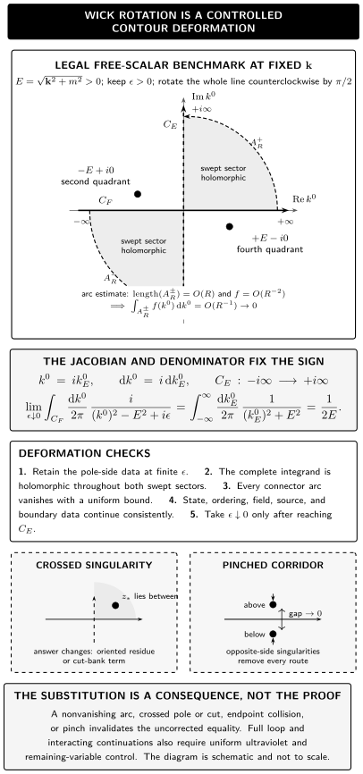
For the free massive scalar, the counterclockwise real-to-imaginary deformation avoids the Feynman poles and , and the integrand makes the quarter-circle contributions vanish. A crossed pole adds a residue, a cut requires a chosen continuation, and a pinch can eliminate the path entirely. The figure is schematic and not to scale; it does not assert an automatic Lorentzian–Euclidean equivalence.
| Figure element | Mathematical statement | Failure meaning |
|---|---|---|
| real contour | , oriented from to | removing first leaves poles on the boundary path |
| rotated contour | , oriented from to | reversing orientation changes the Jacobian sign |
| clear quadrants I and III | the entire swept region is holomorphic | an added pole or cut changes the answer or blocks the move |
| vanishing quarter arcs | the free integrand is | insufficient or nonuniform decay leaves an extra contribution |
| poles in II and IV | selected-vacuum Feynman boundary data | another prescription has different pole geometry |
| pinch warning | singularities approach from opposite sides | no admissible contour remains between them |
Schwartz works the pole geometry, Jacobian, and Euclidean denominator in Schwartz 2014, Appendix B.2, pp. 823–825. Weinberg independently fixes the upward imaginary-axis orientation and emphasizes that divergent loop integrals need a regulator before rotation in Weinberg 1995, § 11.2, pp. 475–476. Weinberg uses the mostly-plus metric and writes the scalar denominator as . With , this differs by an overall minus from the site denominator ; the Feynman pole quadrants, , and upward imaginary-axis orientation are unchanged. Neither one-denominator calculation is a theorem for arbitrary multipoint functions.
Complex time remembers the operator order
Section titled “Complex time remembers the operator order”Use the mixed Euclidean Fourier convention
The Euclidean kernel is
Its contact normalization provides an independent check:
and therefore
The absolute value is a warning: this expression is not one holomorphic function through . It is assembled from two analytic branches,
and
Their Lorentzian boundary values are different operator orders:
The time-ordered and opposite-order correlators are then assembled as
Thus
but the double arrow abbreviates two half-plane continuations plus their boundary prescriptions. It is not substitution into the nonanalytic absolute-value expression at coincidence. In full position space, coincidence and the complexified light cone supply the corresponding singular loci. The spectrum condition is what supports the appropriate time-tube analyticity in the general vacuum framework; the theorem-level domains and distributional boundary construction belong downstream.
The action, field, and source rotate together
Section titled “The action, field, and source rotate together”The energy-contour calculation checks a covariance. A functional formulation must also continue the coordinate, scalar field, source, action, boundary data, and regulated integration cycle.
For the present scalar convention, take
Starting from
the continued contour gives
where
Consequently,
For a regulated scalar interaction analytic along the chosen field contour, adding to the Lorentzian Lagrangian adds to the Euclidean action:
Real-cycle damping requires the regulated Euclidean action to be bounded below with sufficient growth along the retained directions. Even then, the formal map proves neither existence of an interacting continuum measure nor a Lorentzian–Euclidean reconstruction theorem. An unbounded or complex action may require a different integration cycle, and in some cases no corresponding real-cycle continuation exists. The positive scalar-action check is developed in Srednicki 2007, § 29, pp. 185–186; his displayed Euclidean source uses the opposite sign, so that source convention is not imported here.
The site’s Lorentzian source appears with a plus sign in the exponent. Define the scalar Euclidean source on the continued contour by
This formula assumes that belongs to a source family analytic in the required complex-time domain, or that one first forms suitably smeared Lorentzian correlators and then continues those distributions. A generic function specified only on real time has no automatic pointwise value at .
Then
Lorentzian source differentiation inserts , while Euclidean differentiation of this convention inserts . That normalization change follows from the continued exponent and must not be erased by giving both sources the same letter.
At a finite regulator, the statement also requires a mapped integration cycle and compatible endpoint or vacuum data. Writing without such a construction is a mnemonic, not a measure theorem. Zinn-Justin gives the Euclidean scalar action, correlation and source functionals, vacuum interpretation, and ultraviolet qualification in Zinn-Justin 2021, § 6.5, pp. 118–120, while explicitly retaining the need for limiting definitions in continuum field theory.
The scalar rule is not a componentwise rule for every field. Time components of vectors and tensors, spinors and their gamma matrices, derivative insertions, gauge-fixing sectors, and sources dual to those objects acquire their own continuation factors. Each pairing must be checked so the full source term and kinetic operator transform consistently.
Spectral information extends the two-point check
Section titled “Spectral information extends the two-point check”The free calculation is not the only controlled two-point continuation. For a vacuum-subtracted Hermitian scalar operator in a positive physical Hilbert space, a suitably subtracted Källén–Lehmann representation has the form
If the subtractions and spectral integral obey bounds uniform in the deformation, each spectral kernel continues to
The local polynomial is the separately continued contact/subtraction data; it is not determined by the nonlocal spectral measure alone. This extension uses the same positive-energy support that underlies complex-time analyticity. The exact hypotheses and operator-dependent normalization are developed in The Källén–Lehmann Representation.
For the same raw-correlator and source convention, the local part obeys
when that polynomial continuation is admitted. This relation records the phase that the spectral denominator alone cannot determine.
This two-point argument does not rotate a general interacting multipoint function. Several energies are constrained by conservation, singularities move with external kinematics, cuts require specified sheets, and poles or branch surfaces may pinch the available contour. Ultraviolet divergent loop expressions must be regulated before a contour theorem can be applied. Exceptional momenta, massless infrared sectors, unstable backgrounds, and gauge-dependent auxiliary correlators can require different objects or additional prescriptions.
Obstructions and the stop rule
Section titled “Obstructions and the stop rule”Use the following procedure for a proposed continuation.
- Name the target. Specify the Lorentzian state, operator order, external kinematics, source convention, and boundary value.
- Retain the regulator. Keep and any ultraviolet, volume, or infrared regulator until the deformation and its estimates are complete.
- Map the analytic domain. Locate poles, branch points, chosen cuts, endpoints, and singularities that depend on the remaining variables.
- Draw an oriented homotopy. State exactly which region each contour segment sweeps and which sheet it occupies.
- Stop at an obstruction. A crossed isolated pole requires its residue; a crossed cut requires its discontinuity and sheet data; a pinch or trapped endpoint may make the deformation impossible.
- Bound every arc. Prove decay in the swept sector, uniformly in variables or limits that remain.
- Continue all data. Transform coordinates, components, fields, sources, boundary states, and the regulated integration cycle together.
- Take limits in order. Record when , , regulator removal, infinite volume, and external continuation occur.
- Round-trip the answer. Recover the original Lorentzian poles, normalization, and operator ordering from the appropriate boundary approach.
There are three legitimate outcomes: equality by deformation, equality plus explicit residue or discontinuity terms, and failure because no admissible deformation exists. Silently redrawing the contour is not a fourth outcome.
Finite temperature is also a different problem. Compact imaginary time, periodic or antiperiodic boundary conditions, KMS analyticity, and Matsubara frequencies are additional state data, not consequences of the vacuum rotation above. Likewise, finite-time density matrices and nonequilibrium expectation values require a real-time contour rather than an automatic Euclidean replacement.
What Euclidean continuation does not reconstruct
Section titled “What Euclidean continuation does not reconstruct”The free contour produces a Euclidean covariance and checks its return to the selected Lorentzian boundary values. It does not show that an arbitrary collection of Euclidean functions comes from a relativistic QFT. Reconstruction requires a compatible hierarchy and further regularity, Euclidean covariance, symmetry, reflection positivity, growth, and clustering conditions, followed by a theorem that constructs the Hilbert space, fields, spectrum, and Lorentzian boundary values.
The first Osterwalder–Schrader paper places reflection positivity inside that larger package in Osterwalder and Schrader 1973, § 3, pp. 87–90 (Open PDF). Its theorem must be read with the extension and correction in Osterwalder and Schrader 1975, introduction, pp. 281–283, and § IV.1, pp. 287–288 (Open PDF). This page uses neither result as permission to rotate an obstructed perturbative contour.
Check your understanding
Section titled “Check your understanding”1. Track every sign in the free contour
Section titled “1. Track every sign in the free contour”Starting from , set . Why is the Euclidean numerator positive?
Answer
The measure gives , so the original numerator contributes . The denominator becomes . The two minus signs cancel, leaving and then the positive Euclidean kernel as .
2. Recover the operator orders
Section titled “2. Recover the operator orders”Which boundary approaches to and give and , and how is assembled?
Answer
Approaching the imaginary axis from gives ; approaching from gives . Then . Reversing those time sectors gives opposite ordering.
3. Diagnose a failed rotation
Section titled “3. Diagnose a failed rotation”Suppose an additional pole lies in quadrant I, or two moving poles pinch the contour from opposite sides. What may be concluded?
Answer
Crossing the isolated quadrant-I pole changes the result by the oriented residue, so the naïve equality fails. At a pinch, no contour with the required endpoints remains in the nonsingular domain; the proposed deformation is unavailable unless the physical problem itself is changed.
4. Separate continuation from reconstruction
Section titled “4. Separate continuation from reconstruction”Does the successful free-scalar contour prove reflection positivity or the Osterwalder–Schrader theorem?
Answer
No. It verifies one covariance and its boundary values. Reflection positivity is an additional condition on a Euclidean hierarchy, and reconstruction uses it together with the remaining regularity, covariance, symmetry, growth, and clustering hypotheses.
Where to continue
Section titled “Where to continue”- Euclidean Correlators and Schwinger Functions develops the Euclidean hierarchy and its source grammar.
- Contour Deformation, Pinches, and Causal Prescriptions supplies the general homotopy, residue, arc-estimate, and pinch mathematics used here.
- Analytic Continuation between Euclidean and Lorentzian Domains gives the theorem-level complex spacetime domains and distributional boundary statements.
- Reflection Positivity within Osterwalder–Schrader Reconstruction develops the physical reflection form and inventories the other reconstruction hypotheses.
References
Section titled “References”-
Osterwalder, Konrad, and Robert Schrader. “Axioms for Euclidean Green’s Functions.” Communications in Mathematical Physics 31 (1973): 83–112. DOI. Open PDF.
-
Osterwalder, Konrad, and Robert Schrader. “Axioms for Euclidean Green’s Functions II (with an Appendix by Stephen Summers).” Communications in Mathematical Physics 42 (1975): 281–305. DOI. Open PDF.
-
Schwartz, Matthew D. Quantum Field Theory and the Standard Model. First ed. Cambridge: Cambridge University Press, 2014. DOI.
-
Srednicki, Mark. Quantum Field Theory. Cambridge: Cambridge University Press, 2007. DOI.
-
Weinberg, Steven. The Quantum Theory of Fields. Volume I: Foundations. First ed. Cambridge: Cambridge University Press, 1995. DOI.
-
Zinn-Justin, Jean. Quantum Field Theory and Critical Phenomena. Fifth ed. Oxford: Oxford University Press, 2021. DOI.
Original QFT.org content:CC BY 4.0, unless an item supplies different terms. Third-party material retains its own terms.