The Källén–Lehmann Representation

For a vacuum-subtracted Hermitian scalar operator in a positive physical Hilbert space, a normalized Poincaré-invariant vacuum, unitary translations with spectrum in the closed forward cone, completeness, and sufficient distributional regularity yield a nonnegative invariant-mass measure. Vacuum time ordering turns each mass shell in that measure into the same free Feynman kernel. When the chosen time-ordered extension needs no additional local term,

$$\boxed{ \widetilde D_{F,\mathcal O}(p) =\int_{[0,\infty)} \rho_{\mathcal O}(\mathrm d\mu^2) \frac{i}{p^2-\mu^2+i0} }.$$

Neither completeness nor positivity fixes the $+i0$: it records the vacuum time ordering. Microcausality is not used in the scalar two-point completeness or mass-superposition argument. The result does not establish full operator locality, higher-point reconstruction, or scattering theory, and separately renormalized composite time-ordered products can add local contact terms.

Required background. Spectral Decomposition of Two-Point Functions supplies the positive Wightman invariant-mass measure, its forward support, and its discrete and continuous normalization; this page begins from that result.

Helpful background. Spectra, Resolvents, Spectral Measures, and Functional Calculus supplies the measure and boundary-value language used to interpret the resulting integral.

The scalar Källén–Lehmann theorem

Let

$$\widehat{\mathcal O} =\mathcal O -\langle\Omega|\mathcal O|\Omega\rangle\mathbf 1$$

be a Hermitian scalar operator-valued distribution. Define its vacuum Wightman and time-ordered two-point distributions by

$$\begin{aligned} W_{\mathcal O}(x) &=\langle\Omega| \widehat{\mathcal O}(x)\widehat{\mathcal O}(0) |\Omega\rangle, \\ D_{F,\mathcal O}(x) &=\langle\Omega| \mathrm T\!\left\{ \widehat{\mathcal O}(x)\widehat{\mathcal O}(0) \right\}|\Omega\rangle. \end{aligned}$$

The notation $D_F$ is deliberate: it denotes the time-ordered correlator. On the free Gaussian page, $G_F=P_F^{-1}=iD_F$; here $D_{F,\mathcal O}$ is not generally the inverse of a fixed differential operator.

Scalar Källén–Lehmann theorem, in the physical two-point setting. Assume:

1. $|\Omega\rangle$ is a normalized Poincaré-invariant vacuum;
2. translations are unitary with self-adjoint generators $P^\mu$, and their joint spectrum lies in $\overline V_+$;
3. the physical Hilbert-space inner product is positive and the relevant energy–momentum states are complete, equivalently described by the joint spectral resolution of $P^\mu$;
4. $\widehat{\mathcal O}$ is Hermitian and transforms as a scalar; and
5. the distributions are regular enough for the spectral integral, time ordering, Fourier transformation, and the declared coincident-point extension.

Vacuum subtraction removes the contribution of the selected vacuum. We also assume that no other translation-invariant vector has nonzero overlap with $\widehat{\mathcal O}|\Omega\rangle$; if such a contribution is present, its distribution supported at $p=0$ must be displayed separately rather than folded into the ordinary mass-shell measure below.

Then the preceding page gives a positive measure $\rho_{\mathcal O}(\mathrm d\mu^2)$ on $[0,\infty)$ with

$$W_{\mathcal O}(x) =\int_{[0,\infty)} \rho_{\mathcal O}(\mathrm d\mu^2) \Delta_+(x;\mu^2).$$

If the chosen time-ordered extension has no extra local term and the superposition exists as a distribution, then

$$\begin{aligned} D_{F,\mathcal O}(x) &=\int_{[0,\infty)} \rho_{\mathcal O}(\mathrm d\mu^2) \Delta_F(x;\mu^2), \\ \widetilde D_{F,\mathcal O}(p) &=\int_{[0,\infty)} \rho_{\mathcal O}(\mathrm d\mu^2) \frac{i}{p^2-\mu^2+i0}. \end{aligned}$$

Here $\rho_{\mathcal O}(\mu^2)\,\mathrm d\mu^2$ is shorthand for a measure; it can contain Dirac atoms and need not possess an ordinary density everywhere. The assumptions and conclusion are a bounded physical theorem, not a claim that an interacting continuum theory has been constructed from first principles. Schwartz 2014, § 24.2.1, pp. 467–469 gives the modern scalar derivation, while Lehmann 1954, § 1(a), pp. 343–347 develops the propagation-function representation from intermediate states.

Time ordering the mass-shell measure

For a bosonic scalar and $x\ne0$, vacuum time ordering says

$$D_{F,\mathcal O}(x) =\theta(x^0)W_{\mathcal O}(x) +\theta(-x^0)W_{\mathcal O}(-x).$$

Insert the Wightman mass superposition:

$$\begin{aligned} D_{F,\mathcal O}(x) &=\int_{[0,\infty)} \rho_{\mathcal O}(\mathrm d\mu^2) \bigl[ \theta(x^0)\Delta_+(x;\mu^2) \\ &\qquad +\theta(-x^0)\Delta_+(-x;\mu^2) \bigr]. \end{aligned}$$

The bracket is the free Feynman distribution of mass $\mu$,

$$\Delta_F(x;\mu^2) =\theta(x^0)\Delta_+(x;\mu^2) +\theta(-x^0)\Delta_+(-x;\mu^2).$$

Thus the interacting or composite two-point function is not replaced by one free propagator. It is a positive superposition of free-mass two-point distributions, with all theory- and operator-dependent information stored in $\rho_{\mathcal O}$, plus any separately declared local extension term.

The common +i0 denominator

For fixed $\mu$ and spatial momentum $\mathbf p$, let

$$E_{\mu,\mathbf p} =\sqrt{\mathbf p^2+\mu^2}.$$

The energy integral obeys

$$\begin{aligned} &\int_{-\infty}^{\infty}\frac{\mathrm dp^0}{2\pi}\, \frac{i\,e^{-ip^0t}} {(p^0)^2-E_{\mu,\mathbf p}^2+i0} \\ &\qquad= \frac{1}{2E_{\mu,\mathbf p}} \left[ \theta(t)e^{-iE_{\mu,\mathbf p}t} +\theta(-t)e^{+iE_{\mu,\mathbf p}t} \right]. \end{aligned}$$

For $t>0$, the Fourier exponential closes the contour below and selects the positive-energy pole at $p^0=+E_{\mu,\mathbf p}-i0$. For $t<0$, it closes above and selects the negative-energy pole at $p^0=-E_{\mu,\mathbf p}+i0$. Restoring the spatial transform gives

$$\boxed{ \Delta_F(x;\mu^2) =\int\frac{\mathrm d^4p}{(2\pi)^4}\, \frac{i\,e^{-ip\cdot x}} {p^2-\mu^2+i0} }.$$

Every mass shell inherits the same boundary prescription because every term comes from the same vacuum time ordering. A retarded, advanced, thermal, or in–in object requires a different ordering or state construction; positivity of $\rho_{\mathcal O}$ alone does not select any of them.

Composite time ordering and local terms

The Wightman measure is fixed by separated-point matrix elements. Extending a singular composite time-ordered product to $x=0$ is additional data. Two valid extensions can differ by a distribution supported at the origin,

$$C_{\mathcal O}(x) =\sum_{k=0}^{N-1}c_k\Box^k\delta^{(4)}(x),$$

whose Fourier transform is a Lorentz-invariant polynomial $P_{N-1}(p^2)$. If the unsubtracted spectral integral grows too strongly in the ultraviolet, choose a spacelike subtraction point $z_*<0$ and an integer $N\ge1$ large enough to write

$$\begin{aligned} \widetilde D_{F,\mathcal O}^{\mathrm{ren}}(p) &=P_{N-1}(p^2) \\ &\quad+i(p^2-z_*)^N \int_{[0,\infty)} \frac{\rho_{\mathcal O}(\mathrm d\mu^2)} {(\mu^2-z_*)^N(p^2-\mu^2+i0)}. \end{aligned}$$

The polynomial coefficients are fixed by the chosen extension or renormalization conditions, not by positivity of the spectral measure. The nonlocal boundary value still uses the same $\rho_{\mathcal O}$. In the unsubtracted case, omit this polynomial-and-remainder decomposition; with no additional contact term, the result is the theorem stated above.

The previous page’s free composite $\mathcal O=:\!\phi^2\!:$ makes the need visible: its density tends to a constant at large invariant mass, so the formal unsubtracted integral is logarithmically ultraviolet divergent. One subtraction gives a well-defined nonlocal spectral term, while a local constant remains convention dependent.

One-particle weight, continuum, and normalization

In the simplest channel containing one isolated stable scalar and higher-mass continuum,

$$\rho_{\mathcal O}(\mathrm d\mu^2) =Z_{\mathcal O}\delta(\mu^2-m^2)\,\mathrm d\mu^2 +\theta(\mu^2-s_0) \rho_{\mathrm{cont}}(\mu^2)\,\mathrm d\mu^2,$$

where $Z_{\mathcal O}>0$ for nonzero vacuum-to-particle overlap, $\rho_{\mathrm{cont}}\ge0$, and $s_0$ is the lightest allowed continuum threshold in the operator’s channel. The representation separates accordingly:

$$\boxed{ \widetilde D_{F,\mathcal O}(p) =\frac{iZ_{\mathcal O}}{p^2-m^2+i0} +i\int_{s_0}^{\infty}\mathrm d\mu^2\, \frac{\rho_{\mathrm{cont}}(\mu^2)} {p^2-\mu^2+i0} }.$$

The two contributions may coexist. The weight $Z_{\mathcal O}$ is the squared overlap defined on the previous page, not the source functional $Z[J]$. Under $\mathcal O\mapsto c\mathcal O$, both $Z_{\mathcal O}$ and $\rho_{\mathrm{cont}}$ scale by $|c|^2$. No unit total weight or upper bound on $Z_{\mathcal O}$ follows for an arbitrary operator.

The figure shows exactly which normalization and positivity statements accompany this split. Inspect the isolated atom and continuum together, then read the two qualifications below them.

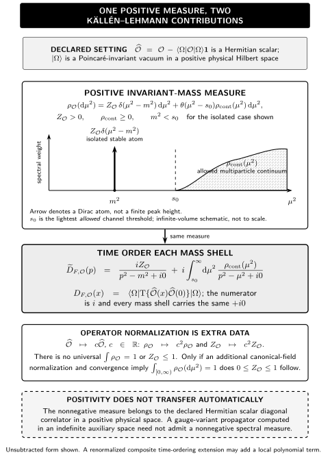
In the simplest scalar channel, nonnegative isolated weight $Z_{\mathcal O}\delta(\mu^2-m^2)$ may coexist with nonnegative continuum support beginning at $s_0$. Both weights depend on operator normalization; only a canonically normalized field with the stated equal-time commutator yields $\int\rho=1$ and $0\le Z\le1$. Positivity does not transfer automatically to a gauge-variant propagator in an indefinite auxiliary space. The diagram is schematic and not to scale.

The same content is available without the figure.

Feature or assumption	Licensed statement	Qualification
Isolated scalar atom	$Z_{\mathcal O}\delta(\mu^2-m^2)$ with $Z_{\mathcal O}\ge0$	It is present only for nonzero overlap with that stable state
Continuum from $s_0$	$\rho_{\mathrm{cont}}(\mu^2)\ge0$ in the declared scalar physical channel	$s_0$ is channel dependent; atoms and continuum may coexist
Operator rescaling	$\rho_{c\mathcal O}=	c
Canonical equal-time commutator	$\int\rho_\phi=1$, hence $0\le Z_\phi\le1$	This is an additional field-normalization sum rule, not a consequence of positivity alone
Gauge-variant component in an indefinite auxiliary space	No automatic nonnegative scalar density	A Hermitian gauge-invariant scalar acting in the positive physical space is not excluded by this warning

For a scalar field with standard kinetic normalization, so that $\pi=\partial_0\phi$, and with the canonical equal-time commutator

$$[\phi(t,\mathbf x),\pi(t,\mathbf y)] =i\delta^{(3)}(\mathbf x-\mathbf y),$$

the spectral commutator gives an additional sum rule. Define

$$\mathcal C_\phi(x) =\langle\Omega|[\phi(x),\phi(0)]|\Omega\rangle =\int_{[0,\infty)} \rho_\phi(\mathrm d\mu^2) \left[ \Delta_+(x;\mu^2)-\Delta_+(-x;\mu^2) \right].$$

Differentiate at equal time. The canonical commutator gives the left side, while every free-mass commutator gives the same delta distribution on the right:

$$-i\delta^{(3)}(\mathbf x) =-i\delta^{(3)}(\mathbf x) \int_{[0,\infty)} \rho_\phi(\mathrm d\mu^2).$$

Therefore, when this canonical normalization and the integral exist,

$$\boxed{ \int_{[0,\infty)} \rho_\phi(\mathrm d\mu^2)=1, \qquad 1=Z_\phi+ \int_{s_0}^{\infty}\mathrm d\mu^2\, \rho_{\mathrm{cont}}(\mu^2), \qquad 0\le Z_\phi\le1 }.$$

This conditional normalization is derived in Schwartz 2014, § 24.2.2, pp. 470–471. Källén’s original analysis connects positive spectral weighting with field-strength renormalization under its conventions Källén 1952, “General Properties of the Operators” and “Definition of the Constant L,” pp. 419–426 (PDF). A composite operator or a rescaled field does not inherit this sum rule automatically.

The role—and nonrole—of locality

The logical chain so far uses no microcausality axiom:

$$\begin{aligned} &\text{invariant vacuum + unitary translations + spectrum condition} \\ &\qquad\Longrightarrow \text{forward spectral support}, \\[2pt] &\text{completeness + Hermiticity + positive norm} \\ &\qquad\Longrightarrow \text{nonnegative spectral weights}, \\[2pt] &\text{scalar Poincaré covariance} \Longrightarrow \text{invariant-mass decomposition}, \\[2pt] &\text{vacuum time ordering} \Longrightarrow \text{common Feynman boundary value}. \end{aligned}$$

For spacelike $x$, a proper orthochronous Lorentz transformation maps $x$ to $-x$. Scalar covariance therefore gives $W_{\mathcal O}(x)=W_{\mathcal O}(-x)$ at the two-point level, so the time-ordering formula is covariant without inserting microcausality as a separate step. Equivalently, every free-mass commutator in the superposition vanishes at spacelike separation.

This conclusion is only about the vacuum expectation of a two-point commutator. It does not prove the operator identity $[\mathcal O(x),\mathcal O(y)]=0$ at spacelike separation, locality of mixed operators, causal factorization, the covariance of all higher time-ordered products, or the existence of scattering states. The conditional sum rule above also uses a separate equal-time canonical commutator; it is not part of the minimal representation theorem.

Positivity, Spectrum, Covariance, and Locality Hypotheses separates those assumptions at theorem level. The Wightman Reconstruction Theorem addresses reconstruction from a complete compatible hierarchy, not from one two-point function alone.

Free and interacting scalar checks

For the canonically normalized free real scalar,

$$\rho_0(\mathrm d\mu^2) =\delta(\mu^2-m^2)\,\mathrm d\mu^2.$$

The theorem immediately returns the site’s free checkpoint,

$$\widetilde D_F^{(0)}(p) =\frac{i}{p^2-m^2+i0}.$$

It also saturates the canonical sum rule: $Z=1$ and there is no continuum in the two-point function of the linear free field.

For an interacting scalar channel with an isolated stable state, the atom-plus-continuum formula above is the first nontrivial application. At spacelike momentum $p^2=-Q^2$ and under the canonical unsubtracted sum rule,

$$\widetilde D_F(-Q^2) =-i\int_{[0,\infty)} \frac{\rho_\phi(\mathrm d\mu^2)} {Q^2+\mu^2} \sim -\frac{i}{Q^2} \qquad(Q^2\to\infty),$$

provided the limit may be interchanged with the spectral integral. The coefficient reproduces the unit total spectral weight. This asymptotic check is not available for an arbitrarily normalized composite operator and must be modified when subtractions are required.

Srednicki 2006 manuscript, § 13, pp. 106–108 (PDF) gives the interacting scalar application in a mostly-plus convention with a differently normalized propagator. For equal contravariant components, $k_{mathrm{Sr}}^2=-p_{mathrm{site}}^2$ and $e^{ik\cdot_{mathrm{Sr}}x}=e^{-ip\cdot_{mathrm{site}}x}$, while $\Delta_{mathrm{Sr}}=iD_{F,\mathrm{site}}$. Hence $1/(k_{mathrm{Sr}}^2+\mu^2-i0)=-1/(p_{mathrm{site}}^2-\mu^2+i0)$, and the two convention factors recover the site’s $i/(p^2-\mu^2+i0)$. The isolated mass contribution has the same physical location and residue after this translation.

Where positivity does not transfer

Changed setting	What survives	What must be rederived
Hermitian scalar in the positive physical Hilbert space	Nonnegative diagonal spectral measure and the scalar representation	Any canonical total-weight sum rule
Non-Hermitian operator	Positivity for the diagonal pairing $\langle\mathcal O(x)\mathcal O^\dagger(0)\rangle$ under the same physical assumptions	A correlator with a different operator ordering or pairing
Operator multiplet	A positive-semidefinite matrix-valued measure	Entrywise positivity of off-diagonal components
Gauge-variant field in an indefinite auxiliary space	A useful gauge-fixed propagator may still exist	Nonnegative spectral density and direct physical-state interpretation
Ghost field	Gauge-fixed correlation functions and BRST bookkeeping	Positive-norm spectral weights
Thermal or other non-vacuum state	State-specific spectral relations can be constructed	The vacuum support, ordering, and positivity argument used here
Composite time-ordered product	The separated-point Wightman measure and nonlocal spectral part	Contact terms, subtractions, and their renormalization conditions

Covariant Free-Photon Quantization and Propagator gives a concrete gauge-fixed example in which the auxiliary state space is not positive definite. This warning does not deny positivity to gauge-invariant Hermitian scalar operators acting on the physical Hilbert space.

Check your understanding

Recover the $+i0$ sign. For $t>0$, identify which energy pole contributes to the contour integral and verify the time dependence.

Check

The factor $e^{-ip^0t}$ closes the contour in the lower half-plane, selecting $p^0=+E_{\mu,\mathbf p}-i0$. Its residue gives $e^{-iE_{\mu,\mathbf p}t}/(2E_{\mu,\mathbf p})$, the positive-frequency Wightman term required by time ordering.

Test the free round trip. Substitute the free delta measure into the representation.

Check

The $\mu^2$ integration evaluates the kernel at $m^2$, yielding $i/(p^2-m^2+i0)$ with no extra factor of $2\pi$ because that factor was already fixed in the preceding Wightman mass-shell normalization.

Locate the extra assumption behind $Z\le1$. Explain why positivity alone is insufficient.

Check

Positivity only gives $Z\ge0$ and nonnegative continuum weight. The upper bound follows after the canonical equal-time commutator fixes the total measure to one: $1=Z+\int\rho_{\mathrm{cont}}$, hence $Z\le1$.

Diagnose a composite subtraction. Use the large-$s$ behavior of the free $:\!\phi^2\!:$ density from the preceding page.

Check

Because $\rho_{\phi^2}(s)$ approaches a nonzero constant, the unsubtracted integral behaves as $\int^\infty\mathrm ds/s$ and diverges logarithmically. A subtraction makes the nonlocal integral convergent, while a local polynomial term records the extension choice.

From the representation to poles and cuts

The representation has now separated the time-ordered two-point function into an isolated denominator and a continuum integral, with all assumptions and normalization conditions visible. It has not yet analyzed either contribution as a complex function.

Poles, Cuts, Thresholds, and Stable Particles next studies that analytic structure, including the infinite-volume qualification. Resonance sheets, infraparticles, and scattering reduction remain later steps.

The modern compound name joins two historically distinct contributions: Källén’s analysis of positive spectral weights in renormalization constants and Lehmann’s propagation-function construction from intermediate states. The cited original locations support that bounded description; they are not used as substitutes for the derivation above.

References

• Källén, Gunnar. “On the Definition of the Renormalization Constants in Quantum Electrodynamics.” Helvetica Physica Acta 25 (1952): 417–434. Open PDF.

• Lehmann, Harry. “On the Properties of Propagation Functions and Renormalization Constants of Quantized Fields.” Il Nuovo Cimento 11 (1954): 342–357. DOI.

• Schwartz, Matthew D. Quantum Field Theory and the Standard Model. First ed. Cambridge: Cambridge University Press, 2014. DOI.

• Srednicki, Mark. Quantum Field Theory. Author-hosted 2006 manuscript preceding the 2007 Cambridge book edition. University of California, Santa Barbara. Author-hosted PDF.