Boundaries, Variations, and Well-Posed Actions

On a finite region, the bulk equations are only part of the stationary-action problem: the surface variation must also be compatible with the data that are held fixed. A well-posed action, in the sense used here, is differentiable on a declared space of fields and boundary data—after any boundary functional has been included, its surface variation vanishes for every allowed tangent variation or produces an explicitly intended natural boundary equation. This is a variational criterion, not a theorem that the resulting differential equation has a solution, a unique solution, or continuous dependence on its data.

The discussion is limited to smooth classical fields on a finite Minkowski region with fixed, non-null boundary geometry. It treats scalar Dirichlet, Neumann, and Robin choices and the analogous Maxwell potential-versus-flux choice. Null boundaries, corners, varying geometry, full surface-charge constructions, analytic PDE theorems, quantum boundary theories, and holographic renormalization are outside the present scope.

Required background. The Action Principle and Field Equations supplies the bulk–boundary decomposition and scalar and Maxwell surface terms used here.

Helpful background. Weak Solutions, Sobolev Spaces, and Well-Posedness separates analytic PDE well-posedness from the variational question treated here. Differential Forms, Integration, Orientation, and Stokes Theorem supplies the orientation and Stokes-theorem language for directed surface integrals.

Differentiability on the chosen boundary-data space

Let a first-derivative bulk action be supplemented by a boundary functional,

$$S_{\mathrm{tot}}[\Phi] = S_{\mathrm{bulk}}[\Phi] + S_{\partial\Omega}[\Phi].$$

After integrating by parts once, its first variation has the form

$$\begin{aligned} \delta S_{\mathrm{tot}} ={}& \int_\Omega \mathrm d^d x\, \mathcal E_A(\Phi)\,\delta\Phi^A \\ &+ \int_{\partial\Omega} \mathrm d\Sigma_\mu\, \Pi_A^\mu\,\delta\Phi^A + \delta S_{\partial\Omega}. \end{aligned}$$

The last line is a one-form on the space of boundary fields. It must be tested only on variations tangent to the chosen data. For example, the condition $\Phi|_{\partial\Omega}=f$ with fixed $f$ allows variations satisfying $\delta\Phi|_{\partial\Omega}=0$; a condition on normal flux instead permits different tangent variations.

The practical test is therefore:

1. Declare the regularity of the fields, the boundary components, and what data are fixed on each component.
2. Vary the complete bulk action without first imposing the bulk equations.
3. Isolate the surface one-form and restrict it to the allowed tangent variations.
4. If it does not vanish, either narrow the data or add a boundary functional matched to the intended control variable.
5. Vary the new total action again. Stop only when the residual surface term vanishes or its free coefficient is the intended natural boundary equation.
6. Analyze existence, uniqueness, constraints, and stability as a separate PDE problem.

This is the elementary finite-region form of the boundary differentiability condition developed in Harlow and Wu 2020, § 1, pp. 3–4; § 2.2, pp. 9–12. A boundary functional introduced here is a classical part of the variational problem. Calling it a boundary counterterm does not, by itself, mean that it cancels a quantum ultraviolet divergence.

Boundary components play different roles

For a time slab $\Omega=[t_i,t_f]\times\Sigma$, the boundary consists of initial and final caps together with a lateral wall $\Gamma=[t_i,t_f]\times\partial\Sigma$. In an ordinary fixed-endpoint derivation, variations vanish on the caps. A condition imposed on the wall instead specifies how the system interacts with that boundary and can change the theory’s allowed modes and conserved fluxes.

These roles should not be exchanged silently. Fixing data on both time caps is an endpoint variational prescription; it is not the same as supplying Cauchy data on one time slice and evolving them. Conversely, a wall condition that makes the action differentiable need not make the hyperbolic initial-boundary value problem analytically well posed.

Scalar boundary data: Dirichlet, Neumann, and Robin

For a real scalar field,

$$S_\phi = \int_\Omega \mathrm d^d x\, \left[ \frac12\partial_\mu\phi\,\partial^\mu\phi -V(\phi) \right],$$

the full first variation is

$$\begin{aligned} \delta S_\phi ={}&- \int_\Omega \mathrm d^d x\, \bigl(\Box\phi+V'(\phi)\bigr)\delta\phi \\ &+ \int_{\partial\Omega} \mathrm d\Sigma_\mu\, \partial^\mu\phi\,\delta\phi. \end{aligned}$$

Choose a positive scalar measure $\mathrm d\Sigma$ on each boundary face and define $p_\phi$ as the coefficient of the boundary variation,

$$p_\phi\,\mathrm d\Sigma \equiv \mathrm d\Sigma_\mu\,\partial^\mu\phi.$$

The surface one-form is then $\int_{\partial\Omega}\mathrm d\Sigma\,p_\phi\delta\phi$. Several distinct variational problems can be built from it.

Dirichlet data. Fix $\phi|_{\partial\Omega}=f$. Since every allowed variation obeys $\delta\phi|_{\partial\Omega}=0$, the original action needs no additional boundary term.

Natural homogeneous Neumann data. Leave the boundary value of $\phi$ free and add no boundary functional. Stationarity for arbitrary boundary $\delta\phi$ then gives

$$p_\phi=0.$$

The scalar surface coefficient and these Dirichlet and homogeneous Neumann alternatives are displayed in Harlow and Wu 2020, § 3.2, p. 21. The underlying integration by parts is also given in Schwartz 2014, § 3.2, pp. 31–32.

Robin data on a spatial wall. Let $\widehat{\mathbf n}$ be the ordinary outward spatial normal, $\partial_n=\widehat{\mathbf n}\mathbin{\cdot}\boldsymbol\nabla$, and fix the temporal endpoints. The wall part of the bulk variation is

$$\delta S_\phi\big|_\Gamma =- \int_{t_i}^{t_f}\mathrm dt \int_{\partial\Sigma}\mathrm dA\, (\partial_n\phi)\,\delta\phi.$$

For fixed functions $\kappa$ and $j$ on the wall, add

$$S_\Gamma =- \int_{t_i}^{t_f}\mathrm dt \int_{\partial\Sigma}\mathrm dA\, \left( \frac{\kappa}{2}\phi^2-j\phi \right).$$

The residual wall variation becomes

$$\begin{aligned} \delta(S_\phi+S_\Gamma)\big|_\Gamma ={}&- \int_\Gamma \mathrm dt\,\mathrm dA\, \\ &\quad\times \bigl(\partial_n\phi+\kappa\phi-j\bigr) \delta\phi. \end{aligned}$$

Free wall variations therefore produce the Robin equation

$$\partial_n\phi+\kappa\phi=j.$$

This includes prescribed inhomogeneous Neumann data when $\kappa=0$; it is not obtained by imposing $\delta\phi=0$. The formula follows directly by re-varying the displayed action. For a canonically normalized scalar, dimensional consistency gives

$$\begin{aligned} [\phi]&=\frac{d-2}{2}, & [p_\phi]&=[j]=\frac d2, \\ [\kappa]&=1. \end{aligned}$$

There is a further distinction between a natural Neumann equation and fixing the flux as the boundary coordinate. A boundary Legendre transform,

$$S_N = S_\phi - \int_{\partial\Omega} \mathrm d\Sigma\,\phi p_\phi,$$

changes the surface variation from $p_\phi\delta\phi$ to

$$\delta S_N\big|_{\partial\Omega} =- \int_{\partial\Omega} \mathrm d\Sigma\,\phi\,\delta p_\phi.$$

It is therefore adapted to fixed-flux variations $\delta p_\phi=0$. This is not the same variational problem as leaving $\phi$ free and deriving $p_\phi=0$ naturally.

Maxwell potential data and normal field-strength flux

For the Maxwell action,

$$S_M[A] =- \frac14 \int_\Omega \mathrm d^d x\, F_{\mu\nu}F^{\mu\nu},$$

integration by parts gives

$$\begin{aligned} \delta S_M ={}& \int_\Omega \mathrm d^d x\, (\partial_\mu F^{\mu\nu})\delta A_\nu \\ &- \int_{\partial\Omega} \mathrm d\Sigma_\mu\, F^{\mu\nu}\delta A_\nu. \end{aligned}$$

Define the boundary flux coefficient by

$$p_A^\nu\,\mathrm d\Sigma \equiv \mathrm d\Sigma_\mu F^{\mu\nu}.$$

Antisymmetry implies that $p_A^\nu$ has no component normal to a smooth boundary face. Consequently the surface term pairs only with the tangential pullback $i^*\delta A$.

Potential-Dirichlet data. Fix $i^*A$ on the boundary, so $i^*\delta A=0$. No extra boundary functional is required.

Natural flux data. If the tangential components of $A$ vary freely and no boundary functional is added, stationarity gives $p_A^\nu=0$ in every tangential direction.

Prescribed or fixed flux. For a fixed tangential source $q^\nu$, the local boundary coupling

$$S_q = \int_{\partial\Omega} \mathrm d\Sigma\,q^\nu A_\nu$$

changes the coefficient to $-(p_A^\nu-q^\nu)\delta A_\nu$ and hence produces $p_A^\nu=q^\nu$ as a natural boundary equation. Alternatively, the boundary Legendre transform

$$S_{M,N} = S_M + \int_{\partial\Omega} \mathrm d\Sigma\,A_\nu p_A^\nu$$

has residual surface variation

$$\delta S_{M,N}\big|_{\partial\Omega} = \int_{\partial\Omega} \mathrm d\Sigma\,A_\nu\delta p_A^\nu,$$

so it is adapted to $\delta p_A^\nu=0$. The Maxwell surface term and the fixed-pullback option are worked out in Harlow and Wu 2020, § 3.3, p. 22; the source coupling and Legendre transform above follow by direct variation.

Gauge compatibility is an additional test. Fixing $i^*A$ restricts the gauge transformations that preserve the boundary data. The flux $p_A$ is gauge invariant, but a functional containing $A_\nu p_A^\nu$ is not automatically invariant under gauge parameters that remain nontrivial at the boundary. One must restrict the admissible parameters, impose compatible boundary conservation conditions, or supply the appropriate boundary and corner structure. Transformations that preserve the data can still act as physical boundary symmetries rather than redundancies, as explained on Fields, Configurations, Dimensions, and Local Dynamics. The boundary-sensitive gauge qualification is developed in Harlow and Wu 2020, § 3.3, pp. 22–23.

The comparison below should be read across each row: the original surface one-form fixes the sign, the boundary functional changes the control variable or the natural equation, and the allowed tangent variation supplies the final test. The double Maxwell frame and the direct field labels keep the two systems distinct without relying on color.

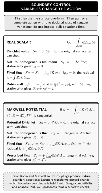
Scalar and Maxwell surface variations require action and boundary data to be chosen together. Dirichlet data kill the original variation, free boundary values produce a natural homogeneous flux equation, Legendre transforms hold flux fixed, and scalar Robin or Maxwell source couplings produce prescribed natural equations. The signs use the page definitions of $p_\phi$ and $p_A^\nu$; the diagram is schematic, assumes a smooth non-null boundary, and does not establish analytic PDE well-posedness or unrestricted boundary gauge invariance.

Field and choice	Boundary functional beyond the bulk action	Allowed tangent variation and residual condition
Scalar Dirichlet	None	$\delta\phi=0$, so $p_\phi\delta\phi$ vanishes
Scalar natural homogeneous Neumann	None	$\delta\phi$ is free, so stationarity gives $p_\phi=0$
Scalar fixed flux	$-\int\mathrm d\Sigma\,\phi p_\phi$	$\delta p_\phi=0$; the residual is $-\int\mathrm d\Sigma\,\phi\delta p_\phi$
Scalar Robin wall	$-\int_\Gamma\mathrm dt\,\mathrm dA\,(\kappa\phi^2/2-j\phi)$	$\delta\phi$ is free, so $\partial_n\phi+\kappa\phi=j$
Maxwell potential Dirichlet	None	$i^*\delta A=0$, so $-p_A^\nu\delta A_\nu$ vanishes
Maxwell natural homogeneous flux	None	Tangential $\delta A$ is free, so $p_A^\nu=0$
Maxwell fixed flux	$+\int\mathrm d\Sigma\,A_\nu p_A^\nu$	$\delta p_A^\nu=0$; the residual is $+\int\mathrm d\Sigma\,A_\nu\delta p_A^\nu$
Maxwell prescribed flux	$+\int\mathrm d\Sigma\,q^\nu A_\nu$	Tangential $\delta A$ is free, so $p_A^\nu=q^\nu$

Variational and analytic well-posedness are different tests

The calculations above answer a question about the first variation: is the action differentiable for the declared fields and boundary data? Analytic well-posedness asks whether the resulting differential equations, together with initial and boundary conditions in specified function spaces,

• admit a solution;
• determine it uniquely, or uniquely modulo a declared gauge redundancy; and
• depend continuously on the data in the chosen norms.

Gauge constraints may impose compatibility conditions before evolution even begins. Estimates may fail for a boundary condition that makes the surface variation vanish. A differentiable action can therefore lead to an empty, nonunique, overdetermined, or unstable solution problem; conversely, a useful PDE formulation need not arise from the particular boundary action chosen here.

The analytic criteria and their function-space dependence are developed on Weak Solutions, Sobolev Spaces, and Well-Posedness. Harlow and Wu likewise separate the Lagrangian boundary condition from existence and uniqueness of the associated initial-value problem in Harlow and Wu 2020, § 2.4, p. 20.

Common pitfalls

Imposing the bulk equations before varying the action. This erases the very surface term that decides which boundary data are admissible. Vary first, retain every boundary contribution, and only then impose stationarity.

Treating all Neumann statements as identical. Free boundary values with the original scalar action yield the natural equation $p_\phi=0$. A Legendre-transformed action instead holds $p_\phi$ fixed and permits nonzero prescribed flux.

Fixing both a field and its normal flux “to be safe.” Those data are independent variational restrictions but are generally too much data for a second-order boundary-value problem. Variational differentiability alone does not certify their analytic compatibility.

Calling every boundary-preserving gauge transformation a redundancy. Some such transformations can carry charges and act physically. The allowed gauge group and the subgroup actually quotiented must be declared separately.

Check your understanding

1. Set $\kappa=0$ in the scalar wall functional and verify the sign of the resulting inhomogeneous Neumann condition.

   Solution

   With $S_\Gamma=\int\mathrm dt\,\mathrm dA\,j\phi$, its variation adds $+\int j\delta\phi$ to the bulk wall term $-\int(\partial_n\phi)\delta\phi$. The residual is $-\int(\partial_n\phi-j)\delta\phi$, so free wall variations give $\partial_n\phi=j$.

2. Show that the Maxwell flux coefficient is tangential to a boundary face.

   Solution

   If $s_\mu$ is proportional to the directed normal covector, then $p_A^\nu\propto s_\mu F^{\mu\nu}$. Contracting again with $s_\nu$ gives $s_\nu s_\mu F^{\mu\nu}=0$ because $s_\nu s_\mu$ is symmetric while $F^{\mu\nu}$ is antisymmetric. Thus the boundary term cannot see the normal component of $\delta A$.

3. Re-vary the scalar Legendre transform and explain why it does not impose $p_\phi=0$.

   Solution

   The original surface term is $p_\phi\delta\phi$. Varying $-\phi p_\phi$ gives $-p_\phi\delta\phi-\phi\delta p_\phi$, so the first pair cancels and the residual is $-\phi\delta p_\phi$. It vanishes because the allowed variations satisfy $\delta p_\phi=0$; the fixed value of $p_\phi$ need not be zero.

The next reorganization is Hamiltonian Initial Data and Phase Space, where cap terms become part of the canonical description. Maxwell constraint reduction continues with The Free Maxwell Field and Gauge Redundancy. Surface charges and their ambiguities belong to Surface Charges, Integrability, and Ambiguities; timelike curved boundaries and renormalized holographic boundary data are treated in Timelike Boundaries, Self-Adjoint Extensions, and AdS Boundary Conditions and One-Point Functions and the Variational Problem.

References

• Harlow, Daniel, and Jie-qiang Wu. “Covariant Phase Space with Boundaries.” Journal of High Energy Physics 2020, no. 10 (2020): 146. DOI.
• Schwartz, Matthew D. Quantum Field Theory and the Standard Model. Cambridge: Cambridge University Press, 2014. DOI.