Lorentzian, Euclidean, and In-In Formulations

Choose the formulation from the physical question and its state or boundary data. In–out transition amplitudes and vacuum time-ordered correlators use Lorentzian in–out boundary conditions; Euclidean Schwinger functions are defined by a Euclidean functional or measure and require a justified continuation before they acquire Lorentzian meaning; causal response is encoded by retarded, advanced, and spectral objects; and expectation values evolved from a specified initial state require an in–in construction. A common denominator or a formal replacement $t=-i\tau$ does not make these objects interchangeable.

The chapter therefore has three main routes: Lorentzian prescriptions and causal response, the Euclidean and reconstruction bridge, and initial-state expectation values with closed-time-path grammar. Match a question to an object · Choose a route · Review the chapter

Enter this chapter

The durable decision sequence is

$$\text{physical question} \longrightarrow \text{state and boundary data} \longrightarrow \text{ordering or contour} \longrightarrow \text{correlator}.$$

Reversing this sequence is the chapter’s characteristic failure mode. Starting from a familiar denominator and adding a mnemonic $i0$, Wick rotation, or doubled field can hide the datum that actually selects the answer.

For the free scalar, the contrast is already visible. With the site’s Lorentzian source sign and selected vacuum,

$$\widetilde D_F(p) =\frac{i}{p^2-m^2+i0}$$

is a vacuum time-ordered correlator, whereas the linear-response kernel is

$$G_{\mathrm{ret}}(x,y) =i\,\theta(x^0-y^0) \langle[\phi(x),\phi(y)]\rangle.$$

The first formula is selected by Feynman boundary data; the second by future support and a commutator. The Euclidean free two-point function instead has

$$\widetilde S_2(p_E)=\frac{1}{p_E^2+m^2},$$

on positive-definite Euclidean momentum space. Relating it to a Lorentzian boundary value requires an analytic domain, a continuation path, compatible state and ordering data, and control of the singularities crossed or avoided.

The Feynman pole placement and distributional equation are checked in Schwartz 2014, § 6.2, pp. 75–77. His Fourier exponential is translated by $k\mapsto-p$, which leaves the denominator and pole locations unchanged. For the response formula, Altland and Simons use the opposite perturbing-Hamiltonian sign; translating their $H_{\mathrm{int}}=+F\phi$ by $F=-J$ to the site’s action source $+J\phi$ produces the displayed $+i$ while preserving future support and spectral analyticity Altland and Simons 2023, § 7.3, pp. 394–402. Zinn-Justin develops the Euclidean functional, scalar correlators, and their vacuum continuation in Zinn-Justin 2021, § 6.5, pp. 118–119; the elementary no-crossed-pole contour check appears in Schwartz 2014, Appendix B.2, pp. 823–825, not as a general continuation theorem.

Match the physical question to the correlator

The figure below is a question-to-object map. Read each row horizontally: the object is fixed jointly by the target quantity and the listed data. The dashed Euclidean–Lorentzian relation is conditional; it is not an equality supplied by renaming time.

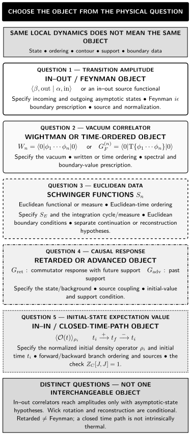
Transition amplitudes, vacuum correlators, Euclidean data, causal response, and initial-state expectation values require different state, ordering, support, or contour information. The Euclidean–Lorentzian bridge is conditional on analytic and reconstruction hypotheses; the other rows are distinctions of physical question, not stages of one automatic conversion. The map is schematic and not to scale.

Physical target	Primary object	Data that select it	What it does not supply by itself
vacuum transition amplitude or time-ordered vacuum data	Lorentzian in–out functional and $D_F$	asymptotic boundary state, time ordering, normalization, and Feynman $i0$	a retarded initial-value response
vacuum correlator in a written operator order	Wightman or ordered correlator	chosen state, field order, and distributional boundary value	a Green inverse merely from its denominator
Euclidean correlation data	Schwinger functions $S_n$	Euclidean action or measure, Euclidean ordering, regularity, and positivity information	Lorentzian reconstruction without the remaining hypotheses
causal linear response	$G_{\mathrm{ret}}$, $G_{\mathrm{adv}}$, and a spectral commutator	state, commutator, support condition, and Fourier boundary value	an in–out amplitude or a thermal interpretation
expectation value from initial data	in–in or closed-time-path functional	normalized initial density operator, initial time, forward and backward branches, and branch sources	thermality unless the initial state satisfies an additional thermal condition

The boundary around this chapter

This chapter develops the physical distinctions and the first free-field checks. It stops before full reconstruction proofs, finite-temperature contour technology, kinetic or stochastic equations, open-system reductions, and cosmological loop applications.

Question beyond this chapter	Developed treatment
Which analytic domains support a theorem-level Euclidean–Lorentzian continuation?	Analytic Continuation between Euclidean and Lorentzian Domains
Which complete Euclidean hypothesis package reconstructs a relativistic theory?	Osterwalder–Schrader Axioms and Reflection Positivity and Osterwalder–Schrader Reconstruction
How are closed-time-path sources used in thermal and nonequilibrium calculations?	Closed-Time-Path Generating Functionals in Practice
How does an in–in effective action produce causal semiclassical backreaction?	In-In Effective Actions and Causal Mean Backreaction

Reflection positivity is one structural condition, not the whole Osterwalder–Schrader theorem. Likewise, a closed time path is a normalized initial-value construction; it is not intrinsically thermal.

The first Osterwalder–Schrader paper places positivity beside distributional regularity, Euclidean invariance, symmetry, and clustering in Osterwalder and Schrader 1973, § 3, pp. 87–90 (Open PDF). Its theorem must be read with the extension and correction in Osterwalder and Schrader 1975, introduction, pp. 281–283, and § IV.1, pp. 287–288 (Open PDF). The overview therefore treats the free reflection test as orientation to a hypothesis package, not as a reconstruction proof.

Check your preparation

The overview has no prerequisite gate. Use these observable checks to decide where to enter.

Can you do this?	Ready	Unsure or repair
Place the Feynman, retarded, and advanced poles and connect them to ordering or support	enter the Lorentzian or causal route	review Scalar Propagators, Ordered Correlators, and Sources and Contour Deformation, Pinches, and Causal Prescriptions
Complete a regulated Gaussian integral and distinguish $e^{iS}$ from $e^{-S_E}$	enter the Euclidean continuation route	repair with Gaussian Fields and Sources
Differentiate a normalized source functional and identify the state and ordering it generates	enter the Schwinger-function or in–in route	repair with The Generating Functional
Insert a complete set of states and interpret a spectral measure	enter the causal/spectral or reflection-positivity branch	repair with Spectral Decomposition of Two-Point Functions and The Källén–Lehmann Representation
Explain the difference between a vacuum vector and a normalized density operator	enter the initial-state route	repair with Vacua, States, and Representations

Choose a route

These are reading routes, not new prerequisite declarations. Follow the hard preparation printed on each page when entering midway.

Goal	Suggested route	Exit capability
Lorentzian boundary values and causal response	boundary conditions → retarded, advanced, and spectral correlators	distinguish frequency boundary data from causal support and choose the correct response object
Euclidean and reconstruction bridge	boundary conditions → Wick rotation → Schwinger functions → reflection positivity	state a valid continuation problem and identify what reflection positivity contributes without claiming the full theorem
Initial-state expectation values	in–out versus in–in → closed-time-path grammar; add causal correlators when interpreting response components	normalize a doubled contour from a specified density operator and identify its four basic components
Inspect contour prescriptions	boundary conditions → pole, residue, and support checks	compare the prescription with the static examples on the theory pages
Inspect a real-time matrix	in–out versus in–in → closed-time-path grammar	compare a Gaussian calculation with the static matrix on the contour-grammar page
Theorem-level Euclidean route	Wick rotation → Schwinger functions → reflection positivity → Mathematical QFT	separate the physical bridge from the hypotheses and proof of reconstruction

Chapter guide

1. Lorentzian Boundary Conditions and the iε Prescription. This page asks how state selection, boundary conditions, convergence factors, and pole displacement distinguish Lorentzian Green functions and amplitudes. It requires the scalar-propagator taxonomy. After it, continue to Wick rotation for Euclidean data or to causal correlators for response.

2. Wick Rotation and Analytic Continuation. This page turns the mnemonic rotation into a contour problem with explicit analytic, spectral, state, ordering, growth, and field-continuation assumptions. It requires the first page and Gaussian source integrals. Continue to Schwinger functions once the free-scalar contour check passes.

3. Euclidean Correlators and Schwinger Functions. This page defines the Euclidean correlation hierarchy, its source grammar, and its relation to the continued free scalar without relabeling it as Lorentzian data. It requires Wick rotation and the generating functional. Continue to reflection positivity when reconstruction is the question.

4. Reflection Positivity within Osterwalder–Schrader Reconstruction. This advanced bridge explains the reflection form and a finite free-scalar matrix test, then inventories the additional hypotheses needed for reconstruction. It requires Schwinger functions; the Källén–Lehmann representation is useful preparation. Continue to Mathematical QFT for the theorem.

5. Retarded, Advanced, and Spectral Correlators. This derivation connects commutators, support, spectral data, and vacuum linear response. It requires Lorentzian boundary prescriptions and spectral decomposition. Continue to Thermal and Nonequilibrium QFT for KMS, transport, and finite-temperature spectral functions.

6. In–Out versus In–In Expectation Values. This page separates asymptotic transition-amplitude data from finite-time expectation values evolved from a specified state or density operator. It requires the generating functional and the state/representation distinction. Continue to the closed-time-path page for branch grammar.

7. Closed-Time-Path Grammar. This page introduces the forward and backward branches, relative action and source signs, initial density insertion, contour ordering, normalization, and four basic two-point components. It requires the in–out/in–in distinction; causal correlators are useful preparation. Continue to the applied real-time formalism in Thermal and Nonequilibrium QFT.

Conventions and continuation hazards

The Lorentzian pages inherit the site’s $(+---)$ metric, Fourier inverse $e^{-ip\cdot x}$, and $+i0$ boundary-value notation. Euclidean pages use a positive-definite metric and $e^{-S_E}$; $p_E^2$ is not a Lorentzian norm with a different sign label.

Three invariants keep translations honest:

• Pole and support check. A convention translation must preserve which side of the energy axis each pole occupies and whether the resulting kernel has future, past, or neither causal support.

• Reflection check. Positivity is tested on the declared positive-Euclidean-time domain after reflection. Ordinary pointwise positivity is neither required nor sufficient.

• Closed-contour check. For a normalized initial density operator and identical branch sources,

  $$Z_{\mathrm{CTP}}[J,J] =\operatorname{Tr}\!\left( U_J(t_f,t_i)\rho_i U_J(t_f,t_i)^\dagger \right) =\operatorname{Tr}\rho_i =1.$$

The last identity follows from unitarity and trace normalization. It does not require a Gibbs state. A thermal contour or KMS relation adds separate conditions.

The normalized trace construction, forward/backward contour, and four branch correlators are developed in Altland and Simons 2023, § 12.2, pp. 705–716. Their Green functions include a conventional overall $-i$ that is not imported into the bare expectation values used here.

The free scalar thread

One scalar example passes through all seven pages while the physical question changes:

1. the two Feynman poles encode vacuum in–out boundary data;
2. a permitted contour deformation produces the Euclidean kernel rather than merely substituting a coordinate;
3. Euclidean source derivatives generate free Schwinger functions;
4. the positive spectral representation supplies a finite reflection-positivity check, not the full reconstruction theorem;
5. the commutator and support condition produce retarded and advanced response;
6. replacing asymptotic boundary states by a specified initial density operator changes the target from an amplitude to an expectation value; and
7. the closed contour organizes the four branch-ordered correlators of a Gaussian initial state.

What stays fixed is the free field, its normalization, and the declared Fourier convention. What changes is the state preparation, ordering, contour, or support condition. That is precisely why algebraically similar kernels answer different questions.

What the seven pages establish together

Statement	Status in this chapter	Missing inference
$i0$ selects a distributional boundary value tied to state and contour data	definition and free energy-plane check	it does not by itself specify every interacting contour deformation
Wick rotation is an analytic continuation problem	physical method with a free-scalar application	it is not a universal theorem for arbitrary correlators or kinematics
Schwinger functions are Euclidean correlation data	primary definition and Gaussian example	they are not automatically Wightman functions
reflection positivity supplies a candidate Hilbert-space positivity form	bounded physical illustration	reconstruction needs the remaining Osterwalder–Schrader hypotheses and proof
retarded and advanced objects encode support-selected response	vacuum causal derivation	a Feynman correlator is not retarded merely because both invert the same operator off shell
in–in and closed-time-path functionals compute initial-state expectation values	foundational semantic distinction and contour grammar	a doubled contour neither assumes thermality nor solves nonequilibrium dynamics

Misconception clinic

“Wick rotation means $t=-i\tau$.” That symbol records only part of a continuation. The analytic domain, contour deformation, state, ordering, field components, sources, growth, and singularity obstructions decide whether the step is valid.

“Euclidean positivity means a positive function.” Reflection positivity is a quadratic form involving Euclidean-time reflection and restricted test data. It is one condition in a larger reconstruction package.

“Feynman means causal.” Feynman ordering implements in–out vacuum boundary data. Retarded support comes from a commutator multiplied by a future-support step function.

“In–in means thermal.” In–in means that the observable is evolved forward and backward from a specified initial state or density operator. A pure vacuum, a Gaussian nonthermal state, and a Gibbs state all fit different choices of that input.

Review the chapter

Review mode	Prompt	Successful answer criterion	Repair
Retrieval	For each of $D_F$, $G_{\mathrm{ret}}$, $S_2$, and $Z_{\mathrm{CTP}}$, name the datum that selects it	names ordering/boundary value, causal support, Euclidean measure/ordering, and initial density plus branches	return to the question map
Explanation	Explain why two kernels with the same off-shell denominator can answer different questions	identifies distinct on-shell boundary terms, support, state, or ordering	review Lorentzian boundary conditions
Derivation check	Continue the free Feynman energy integral only after listing the poles and the deformed contour	no pole is crossed silently and the Euclidean denominator has the correct sign	review Wick rotation
Representation change	Translate the free scalar from Lorentzian $D_F$ to Euclidean $S_2$ and back	recovers the same mass-shell singularity and Feynman boundary value	review Euclidean correlators
Comparison	Distinguish reflection positivity, Hilbert-space positivity, and spectral positivity	gives three different domains and does not use any one as a synonym for the others	review reflection positivity and Källén–Lehmann
Transfer	Choose the object for a compact source switched on after $t_i$ and a field measured later	chooses retarded or in–in response according to whether the target is a response kernel or an initial-state expectation value	review causal correlators and in–out versus in–in
Failure diagnosis	Set $J_+=J_-$ in a normalized closed contour and check the result	obtains $1$ and identifies unitarity plus $\operatorname{Tr}\rho_i=1$	review Closed-Time-Path Grammar
Synthesis	Starting from a Euclidean two-point function, list what must be supplied before claiming a causal real-time prediction	separates analytic continuation, reconstruction hypotheses, state selection, and retarded support	follow the Euclidean route, then the causal page

Continue from this chapter

• Apply real-time contours: Closed-Time-Path Generating Functionals in Practice develops branch sources, Keldysh bases, KMS conditions, kinetics, transport, and open-system applications.
• Develop causal gravitational expectation values: In-In Effective Actions and Causal Mean Backreaction applies the initial-state distinction to semiclassical gravity.
• Enter the Euclidean theorem chain: Euclidean Random Fields and Schwinger Hierarchies and Osterwalder–Schrader Reconstruction supply the theorem-level hypotheses and construction.
• Check the examples: the Lorentzian-boundary and closed-time-path pages provide static pole, residue, support, and Gaussian-matrix benchmarks that can be reproduced independently.
• Return to the volume map: Foundations places this formulation chapter beside the canonical, functional, spectral, and structural routes.

References

• Altland, Alexander, and Ben Simons. Condensed Matter Field Theory. Third ed. Cambridge: Cambridge University Press, 2023. DOI.

• Osterwalder, Konrad, and Robert Schrader. “Axioms for Euclidean Green’s Functions.” Communications in Mathematical Physics 31 (1973): 83–112. DOI. Open PDF.

• Osterwalder, Konrad, and Robert Schrader. “Axioms for Euclidean Green’s Functions II (with an Appendix by Stephen Summers).” Communications in Mathematical Physics 42 (1975): 281–305. DOI. Open PDF.

• Schwartz, Matthew D. Quantum Field Theory and the Standard Model. First ed. Cambridge: Cambridge University Press, 2014. DOI.

• Zinn-Justin, Jean. Quantum Field Theory and Critical Phenomena. Fifth ed. Oxford: Oxford University Press, 2021. DOI.