Closed-Time-Path Generating Functionals in Practice

The closed-time-path generating functional computes expectation values at finite time by evolving a normalized density matrix forward and then backward. Its defining normalization, $Z[J,J]=1$, is the source of causal response and the quickest test of branch signs.

Required background. Review in-out versus in-in expectation values and the closed-time-path grammar.

Helpful background. Thermal density operators and KMS supplies the special equilibrium preparation; the construction below permits any normalized $\rho_0$.

Operator definition and contour orientation

Let $t_0$ be the preparation time and choose $t_f$ later than every operator insertion. With the perturbation written $H_J=H-JO$,

$$Z[J_+,J_-] =\operatorname{Tr}\!\left[ U_{J_+}(t_f,t_0)\rho_0U_{J_-}^{\dagger}(t_f,t_0) \right], \qquad \operatorname{Tr}\rho_0=1.$$

The $+$ branch is time ordered from $t_0$ to $t_f$; the $-$ branch is anti-time ordered on the return. If $J_+=J_-=J$, unitarity gives

$$Z[J,J]=\operatorname{Tr}(U_J\rho_0U_J^\dagger) =\operatorname{Tr}\rho_0=1.$$

The return time is auxiliary: once it lies later than all insertions, forward and backward evolution cancels beyond the latest insertion. The operator construction is used explicitly in Weinberg 2005, § II. An observable dependence on $t_f$ reveals a contour closure or boundary-condition error.

Path-integral form and source rotation

Insert field eigenstates at $t_0$ and $t_f$. For a bosonic field,

$$\begin{aligned} Z[J_+,J_-]={}&\int\mathcal D\phi_+\mathcal D\phi_-\, \langle\phi_+(t_0)|\rho_0|\phi_-(t_0)\rangle\\ &\times\delta[\phi_+(t_f)-\phi_-(t_f)] \exp\!\left\{iS[\phi_+]-iS[\phi_-] +i\int(J_+\phi_+-J_-\phi_-)\right\}. \end{aligned}$$

The minus signs on the return action and source are fixed by orientation. They are not optional conventions once the operator definition has been chosen.

This chapter uses

$$\phi_r=\frac{\phi_++\phi_-}{2},\quad \phi_a=\phi_+-\phi_-,\quad J_r=\frac{J_++J_-}{2},\quad J_a=J_+-J_-.$$

Then the source is $\int(J_a\phi_r+J_r\phi_a)$. A physical perturbation has equal branch sources, hence $J_a=0$ and $J_r=J$. With $Z=e^{iW}$,

$$\frac{\delta W}{\delta J_a}=\langle\phi_r\rangle, \qquad \frac{\delta W}{\delta J_r}=\langle\phi_a\rangle=0 \quad\text{at }J_a=0.$$

This apparently crossed source pairing is what makes derivatives with respect to the physical source generate causal response.

The schematic fixes the logical order of the construction. Follow the solid arrows from the normalized density matrix around the forward and backward histories; the dashed equal-source branch is the quickest test of the contour orientation and source signs.

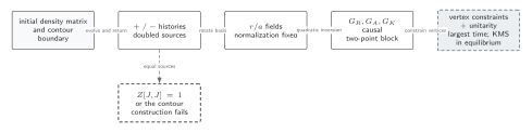
The $+$ branch evolves forward and the $-$ branch returns, so their action and source terms enter with opposite contour orientation. Equal physical sources must give $Z[J,J]=1$ before any $r/a$ rotation is trusted. The propagator labels in later boxes inherit the page’s local field and source normalization; the quadratic-inversion step applies to the two-point block, while interaction vertices come from rotating the action. KMS is an additional equilibrium condition, not a contour identity. The diagram is schematic and not to scale.

The sections Operator definition and contour orientation and Path-integral form and source rotation give the text and equation equivalent of the first three boxes and the normalization branch.

Contour matrix for a Gaussian state

Define

$$G^{ab}(x,y)=-i\langle T_{\mathcal C}\phi_a(x)\phi_b(y)\rangle, \qquad a,b\in\{+,-\}.$$

Writing $G^>(x,y)=-i\langle\phi(x)\phi(y)\rangle$ and $G^<(x,y)=-i\langle\phi(y)\phi(x)\rangle$ gives

$$\begin{aligned} G^{++}&=\theta_{xy}G^>+\theta_{yx}G^<,& G^{--}&=\theta_{yx}G^>+\theta_{xy}G^<,\\ G^{-+}&=G^>,&G^{+-}&=G^<. \end{aligned}$$

Thus $G^{++}+G^{--}=G^{+-}+G^{-+}$, the two-point shadow of $Z[J,J]=1$. Equal-time contact prescriptions must be fixed consistently with the canonical commutator; choosing different $\theta(0)$ values in different components breaks this identity.

For a free oscillator with occupation $n$, $G^>(t,t')=-i[(n+1)e^{-i\omega(t-t')}+ne^{i\omega(t-t')}]/(2\omega)$ and $G^<(t,t')=G^>(t',t)$. Substitution verifies every branch relation and shows explicitly that the state changes Wightman functions without changing contour orientation.

Failure tests

• Set $J_+=J_-$ numerically for an arbitrary time profile and demand $Z=1$, not merely $Z[0,0]=1$.
• Move $t_f$ later; correlators before the old return time must not change.
• Check the branch matrix identity before rotating to $r/a$ variables.
• Distinguish an initial density matrix from vacuum $i\epsilon$ preparation. In-out boundary conditions compute an amplitude, not a finite-time expectation value.
• Preserve any imaginary-time leg or boundary action used to prepare $\rho_0$; silently dropping it changes the state.

Exercise

Differentiate $Z[J_+,J_-]$ with respect to $J_+(x)$ and $J_-(x)$ and show that their sum in the $J_r$ direction vanishes when $J_+=J_-$.

Solution

The return source enters the exponent with the opposite sign. At equal sources, the two derivatives insert the same Heisenberg operator on opposite sides of the trace, and cyclicity makes their oriented sum zero. Equivalently, $J_r$ changes both branch sources equally while $Z[J,J]=1$, so $\delta Z/\delta J_r=0$ and therefore $\langle\phi_a\rangle=0$.

Continue

Encode the preparation through initial contour boundary conditions and turn normalization into exact largest-time identities.

References

• Chou, K.-C., Su, Z.-B., Hao, B.-L., and Yu, L. (1985). “Equilibrium and Nonequilibrium Formalisms Made Unified.” Physics Reports 118, 1–131. DOI.
• Schwinger, J. (1961). “Brownian Motion of a Quantum Oscillator.” Journal of Mathematical Physics 2, 407–432. DOI.
• Weinberg, S. (2005). “Quantum Contributions to Cosmological Correlations.” Physical Review D 72, 043514. arXiv:hep-th/0506236; DOI.

References

Section titled “References”- Crossley, M., Glorioso, P., and Liu, H. (2017). “Effective Field Theory of Dissipative Fluids.” Journal of High Energy Physics 2017(09), 095. arXiv:1511.03646; DOI.