Validity and Breakdown of Kinetic Descriptions

A kinetic solution is credible only when two distinct questions are answered: has the discretized equation been solved accurately, and is that equation a controlled reduction of the parent quantum dynamics? Positivity, exact collision invariants, numerical convergence, shell separation, memory loss, and closure variation test different failure modes and cannot substitute for one another.

Required background. Use quasiparticle shell and gradient counting and collision-kernel conservation.

Helpful background. Numerical Kadanoff–Baym validation provides the parent two-time benchmark.

Two validation layers

Equation-level convergence varies timestep, momentum and angle grids, quadrature, volume, collision cutoffs, delta-function representation, nonlinear tolerance, and tail truncation while holding the physical kinetic model fixed.

Model-level control varies spectral width, gradient order, memory window, initial correlations, scattering/resummation order, moment or matrix closure, and particle basis. A converged solver can produce an inaccurate kinetic model; a controlled model can be implemented badly.

The shared stochastic and kinetic closure table keeps these records separate.

Conservation and positivity

For every collision invariant $\psi_A$,

$$\mathcal R_A(t)=\sum_i\int dP_i\,\psi_{A,i}(p)C_i[f]$$

must vanish analytically and converge to zero numerically. Monitor local and global residuals. A projection that forces $\mathcal R_A=0$ after each step should be reported and tested for its effect on entropy and positivity.

Positivity-preserving limiters can prevent $f<0$, and fermionic solvers must also enforce $f\le1$. But a limiter that clips cells changes moments and collision equilibria. Measure the total clipped weight and show it converges away. Matrix kinetics requires Hermitian positive-semidefinite eigenvalues, not merely positive diagonal entries.

Resolution and collision geometry

Energy delta functions define lower-dimensional manifolds in momentum space. Smearing them by width $\epsilon_\delta$ creates an additional control: the grid must resolve the smear, and observables must stabilize as both grid and $\epsilon_\delta$ are refined in a coordinated limit. Exact reaction parametrizations can conserve better but may have singular Jacobians near thresholds.

Rare high-momentum tails can dominate transport coefficients even when they carry little density. Extend momentum cutoffs while monitoring weighted moments, not only $L^1$ normalization. Soft and collinear regions need matched regulators and subtraction-scale studies.

Stiff collision rates require implicit or exponential integrators. Solver stability at a large timestep does not establish temporal accuracy; recover the method’s convergence order on a nontrivial collision benchmark.

Parent-theory comparison

Compare kinetic and Kadanoff–Baym evolution with matched initial correlators, renormalized parameters, volume, and observables; Stan, Dahlen, and van Leeuwen 2009, §§ II–III provide a concrete two-time propagation benchmark. Useful controls include:

• free streaming, which tests the streaming operator and characteristics;
• exact equilibrium, which tests detailed balance and stationarity;
• a solvable relaxation model with protected zero modes;
• full two-time evolution before shell and Markov reductions; and
• successive effective kinetic orders with the same matching prescription.

Disagreement should be classified: discretization error, finite-width/off-shell effect, memory, initial correlation, missing process, coherence, or uncontrolled coupling. Fitting a relaxation time to the parent curve is calibration, not a predictive validation.

Breakdown indicators

Kinetic theory should be replaced or enlarged when any of the following remains $O(1)$:

$$\frac{\Gamma}{E},\qquad \frac{\Gamma}{\Delta E},\qquad \frac{\tau_{\mathrm{corr}}}{\tau_X},\qquad \frac{\ell_{\mathrm{mfp}}}{L_X},$$

or when spectral peaks disappear, Wigner functions require large negative/coherent components, collision invariants cannot be maintained under the chosen closure, or observables change strongly with memory and gradient order. Critical slowing, strong fields, plasma instabilities, very early times, and nearly degenerate mixing are common boundaries.

“Hydrodynamization” can occur before local equilibrium for selected stress observables, but its time may depend on the model, norm, and tolerance. A solver-dependent crossing of an arbitrary threshold is not a universal physical time.

The map condenses the acceptance sequence into paired assumptions and diagnostics. The four columns are independent: each dashed vertical arrow names a failure mode and points to a relevant test, and no passed column licenses the others.

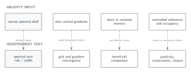
The upper row lists independent assumptions of a kinetic reduction; the lower row lists representative diagnostics. Each vertical dashed link pairs a failure mode with a test, while the absence of horizontal arrows emphasizes that the columns do not imply one another. Passing spectral and grid checks does not prove short memory, controlled coherence, positivity, conservation, or closure accuracy. The diagram is schematic and not to scale.

The sections Two validation layers, Parent-theory comparison, Breakdown indicators, and Reproducible acceptance sequence give the complete text and equation equivalent of both rows.

Reproducible acceptance sequence

1. Verify free streaming and exact equilibrium.
2. Demonstrate discrete collision invariants and entropy behavior.
3. Refine time, momentum, angle, cutoff, delta representation, and tails independently.
4. Quantify limiter or projection intervention.
5. Vary collision and closure order.
6. Test width, gradient, and memory assumptions against the parent theory.
7. Repeat at several parameter points spanning the claimed regime.
8. Report numerical and model discrepancies separately.

Exercise

A positivity limiter changes $10^{-6}$ of total particle number but $5\%$ of a shear-weighted moment. Is the shear result converged?

Solution

No. The small unweighted mass of clipped cells is irrelevant if the target observable emphasizes those cells. The limiter’s effect must converge for the shear moment itself under grid, timestep, and tail refinement.

Continue

This page is the kinetic handoff boundary. Move to hydrodynamics, stochastic dynamics, or phenomenology only with the validated distribution, collision invariants, closure range, and separate numerical/model uncertainty record.

References

• Arnold, P., Moore, G. D., and Yaffe, L. G. (2003). “Effective Kinetic Theory for High Temperature Gauge Theories.” Journal of High Energy Physics 2003(01), 030. arXiv:hep-ph/0209353; DOI.
• Stan, A., Dahlen, N. E., and van Leeuwen, R. (2009). “Time Propagation of the Kadanoff–Baym Equations for Inhomogeneous Systems.” Journal of Chemical Physics 130, 224101. DOI.