Statistical Ensembles and Field Configurations

An equilibrium ensemble is a normalized measure on microscopic field configurations, not a representative field profile. The microcanonical, canonical, and grand-canonical descriptions differ by which extensive data are fixed and which are exchanged with an ideal reservoir. At finite regulator and volume their relation is exact through Laplace transforms; their equivalence after removing the regulator or taking infinite volume is a separate dynamical and convexity question.

The finite-volume ensemble definitions and thermodynamic-limit qualifications used here follow Ruelle 1999, chs. 1–3.

Required background. Probability Spaces, Random Variables, and Conditional Expectation supplies normalized measures and expectations. Hamiltonian Initial Data and Phase Space supplies the field-theory phase space and conserved Hamiltonian. Helpful background. Wick Rotation and Analytic Continuation explains why a Euclidean functional weight is not automatically a Lorentzian probability law.

Ensembles as measures on configurations

Regulate the system in a finite spatial region $V$ with boundary conditions included in the definition of the configuration space $\Omega_V$. A microscopic point $X\in\Omega_V$ may comprise fields and momenta, $(\phi,\pi)$, or a Euclidean field configuration. For reference measure $\mathrm d\nu_V(X)$, an ensemble has density $P(X)$ satisfying

$$P(X)\geq0, \qquad \int_{\Omega_V}\mathrm d\nu_V(X)P(X)=1, \qquad \langle\mathcal O\rangle_P= \int_{\Omega_V}\mathrm d\nu_V(X)P(X)\mathcal O(X).$$

The probability density depends on the chosen reference measure; the probability assigned to a measurable set does not. Constraints such as Gauss’s law, fixed boundary data, or a charge sector must be built into $\Omega_V$, the measure, or explicit delta functions. Integrating over an unconstrained space and imposing the constraint only after normalization generally defines a different ensemble.

For Hamiltonian $H(X)$ and commuting conserved quantities $Q_a(X)$, the standard finite-volume ensembles are

$$\begin{aligned} \rho_{\mathrm{mc}}(X;E,q_a) &=\frac{\delta(H(X)-E)\prod_a\delta(Q_a(X)-q_a)} {\Omega_V(E,q_a)},\\ \rho_{\mathrm c}(X;\beta) &=\frac{e^{-\beta H(X)}}{Z_V(\beta)},\\ \rho_{\mathrm{gc}}(X;\beta,\mu_a) &=\frac{e^{-\beta[H(X)-\sum_a\mu_a Q_a(X)]}} {\Xi_V(\beta,\mu_a)}. \end{aligned}$$

Here $\Omega_V$ is the density of states, while $Z_V$ and $\Xi_V$ normalize the canonical and grand-canonical measures. The symbol $\rho$ in these formulas is a classical density. A quantum statistical operator is developed on Thermal Density Operators and the KMS Condition.

From constrained data to reservoir variables

The canonical partition function is the Laplace transform of the density of states,

$$Z_V(\beta)=\int \mathrm dE\,\Omega_V(E)e^{-\beta E}.$$

Conversely, when the analytic domain and contour are controlled,

$$\Omega_V(E)=\int_{c-i\infty}^{c+i\infty} \frac{\mathrm d\beta}{2\pi i}\,e^{\beta E}Z_V(\beta).$$

This inverse formula is exact at the regulated level; a saddle-point approximation requires large volume and a stable stationary point. If $\Omega_V(E)\asymp e^{V s(e)}$ with $e=E/V$, then the canonical integral is governed by extrema of $s(e)-\beta e$. A unique differentiable maximum gives $\beta=s'(e_*)$. Multiple maxima, nonconcave entropy, long-range interactions, or a boundary-dominated system can invalidate the usual equivalence inference even though the transform itself remains correct.

A regulated scalar-field example

On a spatial lattice with $N$ sites and spacing $a$, take

$$H=\sum_{x}a^{d-1} \left[ \frac12\pi_x^2+\frac12\sum_i(\nabla_i\phi_x)^2 +\frac12m^2\phi_x^2+\frac{\lambda}{4!}\phi_x^4 \right].$$

The canonical measure is the finite-dimensional integral

$$Z_N(\beta)=\int\prod_x\frac{\mathrm d\phi_x\,\mathrm d\pi_x}{2\pi} \,e^{-\beta H[\phi,\pi]}.$$

The chosen normalization of each phase-space cell affects the additive free energy but cancels from normalized field expectations. The regulator, volume, and boundary conditions are nevertheless physical inputs to every finite-$N$ statement. Only after specifying how $a\to0$ and $V\to\infty$ are taken can one claim a continuum or thermodynamic result.

Convention and limit table

This semantic table is the shared reference for the equilibrium and KMS opening arc.

Object	Finite regulated definition	Limit or continuation required	Claim that does not follow automatically
Configuration	$X\in\Omega_V$ with measure, constraints, and boundary data	Regulator removal or infinite-volume construction	That one typical configuration equals the ensemble
Canonical state	$P\propto e^{-\beta H}$, $\beta>0$	Thermodynamic limit at fixed intensive data	Equivalence to a constrained ensemble
Grand-canonical state	$P\propto e^{-\beta(H-\mu_aQ_a)}$	Stability domain and charge-sector control	Existence for arbitrary $\mu_a$
Euclidean weight	$e^{-S_E}$ on a declared integration cycle	Reconstruction hypotheses for Lorentzian theory	Real-time response or unitary evolution
Connected susceptibility	Source derivative or integrated connected correlator	Contact subtraction and limit order	Equality to an unsubtracted zero-momentum correlator
Phase	Selected infinite-volume state or nonanalytic thermodynamic potential	$V\to\infty$ before removing a selecting source	Strict spontaneous breaking at finite $V$
KMS relation	Analytic boundary condition on time-translated observables	Algebra and thermodynamic-limit hypotheses	Existence of a trace-class Gibbs operator
Spectral reconstruction	Estimator acting on finite noisy Euclidean data	Resolution and prior validation	Pointwise or unique real-time spectrum

The table records distinct questions—definition, limiting construction, and inference ceiling—so that a later calculation cannot hide a change of ensemble or order of limits.

Checks and failure modes

Normalization, support, and conserved constraints should be tested before computing observables. For a proposed change of variables, include its Jacobian in the reference measure. For an ensemble comparison, identify the held-fixed extensive or intensive variables. For a field integral, state the ultraviolet regulator and verify that the weight is normalizable; a potential unbounded below does not define a canonical probability measure merely because perturbation theory produces formal diagrams.

Configuration–ensemble confusion. A field configuration can look inhomogeneous while the ensemble is translation invariant. Symmetry is a property of the measure and its moments, not of every sample.

Premature equivalence. The Laplace relation between $\Omega_V$ and $Z_V$ is not a proof that their infinite-volume equations of state coincide. Concavity, additivity, and the relevant limit order must be checked.

The schematic below organizes the relationships used on this page. Inspect it with this question in mind: How do ensembles, partition functions, response derivatives, Legendre transforms, and phase probabilities connect?

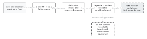
The finite-volume partition function generates response, Legendre transforms change controlled variables, and large-deviation rate functions encode phase weights only after the thermodynamic-limit order is declared. Solid connections show the primary relation; dashed outlines or arrows mark qualifications and failure boundaries. The diagram is schematic and not to scale.

The surrounding discussion supplies the relevant equations and checks in text form; the figure is a navigational summary.

Exercise

Let $H=p^2/2+\omega^2q^2/2$. Compute the canonical covariance and verify equipartition.

Solution

The Gaussian factors give $Z=(\beta\omega)^{-1}$ up to the chosen phase-space normalization. Differentiating the two one-dimensional Gaussians gives $\langle p^2\rangle=1/\beta$ and $\omega^2\langle q^2\rangle=1/\beta$, hence $\langle H\rangle=1/\beta$. The result checks both normalization and the factor of $\beta$ in the weight.

References

• Ellis, Richard S. Entropy, Large Deviations, and Statistical Mechanics. Grundlehren der mathematischen Wissenschaften 271. New York: Springer, 1985. doi:10.1007/978-1-4613-8533-2.
• Kardar, Mehran. Statistical Physics of Fields. Cambridge: Cambridge University Press, 2007. doi:10.1017/CBO9780511815881.
• Ruelle, David. Statistical Mechanics: Rigorous Results. Singapore: World Scientific, 1999. doi:10.1142/4090.