Thermal Spectral Positivity and Sum Rules

For a Hermitian operator acting in a positive Hilbert space, the thermal spectral density is nonnegative at positive frequency and odd in frequency. Equal-time operator algebra and ultraviolet asymptotics can impose moment or subtracted sum rules. Each statement is channel specific: non-Hermitian charged operators require a spectral matrix, gauge-variant fields can violate positive-metric assumptions, and finite density can alter adjoints, detailed balance, and stability domains.

The positivity domain and thermal spectral normalization used here are developed in Le Bellac 1996, ch. 2.

Required background. Thermal Propagators and Spectral Representations fixes $\rho$ and its correlator dictionary. Microcausality and Relativistic Compatibility supplies causal support. Helpful background. Free-Field OPE Preview motivates ultraviolet moment constraints.

Lehmann positivity and its hypotheses

For Hermitian $\mathcal O$ in a finite-volume positive Hilbert space,

$$\rho(\omega)= \frac{2\pi}{Z}\sum_{m,n} \left(e^{-\beta E_m}-e^{-\beta E_n}\right) \lvert\langle m|\mathcal O|n\rangle\rvert^2 \delta(\omega-E_n+E_m).$$

At $\omega>0$, the delta function selects $E_n>E_m$, so the parenthesis is positive. Hence

$$\rho(\omega)\ge0\quad(\omega>0), \qquad \rho(-\omega)=-\rho(\omega).$$

The conclusion used Hermiticity, a positive inner product, a stable Gibbs state, and the same neutral channel on both sides. For operators $A\ne A^\dagger$, the positive object is a matrix of spectral measures tested against $c_iA_i$ and its adjoint, not each off-diagonal component. At finite chemical potential the equilibrium generator and physical frequency must be declared before transferring the sign argument.

BRST gauge fixing introduces negative-norm or unphysical sectors. Gauge-invariant composite observables may recover a positive physical spectral representation, while a gauge-dependent gluon or ghost propagator need not. Positivity is therefore a theorem to be applied after channel qualification, not a generic reconstruction prior.

Equal-time and moment sum rules

From the inverse Fourier transform,

$$\int\frac{\mathrm d\omega}{2\pi}\rho(\omega,\mathbf p) =\langle[\mathcal O(0,\mathbf p),\mathcal O(0,-\mathbf p)]\rangle.$$

For a bosonic operator with itself this vanishes, consistently with oddness. The first moment is

$$\int\frac{\mathrm d\omega}{2\pi}\, \omega\rho(\omega) =\langle[\mathcal O,[H,\mathcal O]]\rangle,$$

provided the moment converges and contact terms are included. For a canonically normalized coordinate $q$ of mass $m$, this yields $1/m$, an $f$-sum-rule prototype.

Higher moments probe nested commutators but often diverge in QFT. A useful sum rule then subtracts a reference spectrum or its known ultraviolet asymptotics:

$$\int_0^\infty\mathrm d\omega\, w(\omega) \left[\rho_T(\omega)-\rho_{\mathrm{ref}}(\omega) -\rho_{\mathrm{asymp}}^{\mathrm{sub}}(\omega) \right]=C.$$

The operator-product expansion can constrain $\rho_{\mathrm{asymp}}$, but Wilson coefficients, condensate conventions, operator mixing, and analytic continuation must be matched. Removing a divergent tail by hand does not create a sum rule.

Susceptibility and low-frequency structure

For a suitable neutral channel with no omitted static term,

$$\chi=\lim_{\mathbf p\to0}G_E(0,\mathbf p) =\lim_{\mathbf p\to0} \int\frac{\mathrm d\omega}{2\pi} \frac{\rho(\omega,\mathbf p)}{\omega}.$$

The integrand is even and nonnegative for a qualified Hermitian channel. Conserved charges can generate delta functions, hydrodynamic poles, or noncommuting $\omega\to0$ and $\mathbf p\to0$ limits. Contact and magnetization contributions are handled explicitly in the transport chapter.

Testing a proposed spectral ansatz

Before accepting $\rho_{\mathrm{ans}}$:

1. identify the operator, adjoint, charge, gauge status, and state;
2. verify oddness or the correct charged-channel relation;
3. test positive-frequency positivity only when its hypotheses hold;
4. impose exact commutator moments with matched contact terms;
5. match ultraviolet asymptotics and the subtraction scheme;
6. check susceptibility and the declared order of limits;
7. verify that poles, cuts, and widths do not double count the same weight; and
8. propagate uncertainty rather than forcing exact constraints known only approximately.

For the free scalar spectral density,

$$\int\frac{\mathrm d\omega}{2\pi}\, \omega\rho_0(\omega,\mathbf p)=1,$$

which matches $[\phi,\dot\phi]=i$ in canonical normalization. This provides a strong normalization check independent of the Euclidean kernel.

Common pitfalls

Positive Euclidean correlator implies positive spectrum. Reflection or pointwise positivity of one Euclidean data vector is not the Lehmann theorem. Qualify the operator and Hilbert-space metric.

A divergent moment treated numerically. Increasing a frequency cutoff can conceal the divergence over a short range. Derive the ultraviolet degree and subtraction before fitting.

A sum rule treated as shape identification. One moment constrains one weighted integral. It does not locate a unique peak or width.

The schematic below organizes the relationships used on this page. Inspect it with this question in mind: What connects thermal correlators, spectral densities, exact continuation, and finite-data reconstruction?

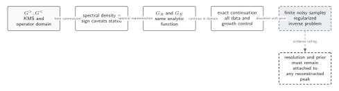
KMS and the commutator determine compatible Euclidean and retarded representations; exact analytic continuation is unique under its hypotheses, whereas reconstructing a spectrum from finite noisy data is an ill-posed inference problem. Solid connections show the primary relation; dashed outlines or arrows mark qualifications and failure boundaries. The diagram is schematic and not to scale.

The surrounding discussion supplies the relevant equations and checks in text form; the figure is a navigational summary.

References

• Kapusta, Joseph I., and Charles Gale. Finite-Temperature Field Theory: Principles and Applications. 2nd ed. Cambridge: Cambridge University Press, 2006. doi:10.1017/CBO9780511535130.
• Le Bellac, Michel. Thermal Field Theory. Cambridge: Cambridge University Press, 1996. doi:10.1017/CBO9780511721700.
• Romatschke, Paul, and Dam Thanh Son. “Spectral Sum Rules for the Quark–Gluon Plasma.” Physical Review D 80 (2009): 065021. doi:10.1103/PhysRevD.80.065021; Open PDF.