Thermal Effective Potentials and Phase Diagrams

A thermal effective potential is a controlled phase-diagram tool only after its effective object, loop order, resummation, counterterms, gauge fixing, and scale dependence are specified. Degenerate background minima can suggest coexistence, but background locations and truncated barriers are not themselves gauge-invariant observables.

Required background. Use the Landau–Ginzburg functional for the coarse-grained interpretation and gauge dependence of thermal observables for perturbative order counting.

Helpful background. Ring and daisy resummation treats the bosonic zero modes that invalidate a naive loop expansion.

Renormalized and resummed construction

For a background $\varphi$, a common perturbative organization is

$$V_{\mathrm{eff}}(\varphi,T)=V_0(\varphi) +V_{1,T=0}(\varphi;\mu) +\Delta V_{1,T}(\varphi,T) +V_{\mathrm{ring}}(\varphi,T)+\cdots .$$

In four dimensions,

$$\Delta V_{1,T}=\frac{T^4}{2\pi^2} \left[\sum_b n_bJ_B(m_b^2/T^2)-\sum_f n_fJ_F(m_f^2/T^2)\right],$$

where the signs and definitions of $J_{B,F}$ must be declared. Bosonic zero modes require screening. In the Arnold–Espinosa organization the leading ring correction is

$$V_{\mathrm{ring}}=-\frac{T}{12\pi}\sum_{b,0}n_b \left([m_b^2(\varphi)+\Pi_b(T)]^{3/2}-[m_b^2(\varphi)]^{3/2}\right).$$

Only screened zero modes belong in this sum. Replacing masses everywhere and also adding the displayed term double counts parts of the resummation; the order-by-order organization is explicit in Arnold and Espinosa 1993, §§ II–III. Dimensional reduction provides a cleaner scale-separated alternative: match a three-dimensional EFT, run or simulate it, and keep hard, soft, and ultrasoft contributions distinct.

Negative field-dependent $m_b^2$ can make a loop potential complex. The imaginary part signals expansion around an unstable homogeneous background, not a decay rate. Taking an absolute value or discarding it silently changes the approximation; a coarse-grained real potential, analytic continuation prescription, or EFT treatment must be justified.

Phase coexistence and thermodynamics

At a candidate first-order transition temperature $T_c$, two equilibrium branches have equal physical free-energy density,

$$f_1(T_c)=f_2(T_c).$$

For a controlled background calculation one often approximates $f_i(T)$ by $V_{\mathrm{eff}}(\varphi_i(T),T)$ evaluated at stationary branches. Thermodynamic derivatives must include the explicit temperature dependence; because $\partial_\varphi V=0$ on an exact stationary branch,

$$s_i=-\frac{df_i}{dT}=-\left.\frac{\partial V_{\mathrm{eff}}}{\partial T}\right|_{\varphi_i}, \qquad L=T_c(s_2-s_1),$$

up to the ordering convention for phases. At finite perturbative order, solving the minimum nonperturbatively in the truncated potential can mix orders. A strict expansion of both $T_c$ and the extrema is often required for gauge-consistent results.

Pressure is $p=-f$, energy density is $e=f+Ts$, and the sound speed requires derivatives along the physical branch. A plotted barrier supplies none of these derivatives automatically.

The diagram separates the construction and comparison of approximate branches from the evidence needed for a physical phase statement. In particular, the barrier in a resummed potential belongs to the metastable branch, not to the exact equilibrium potential.

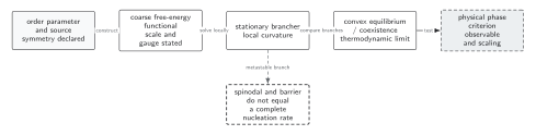
A renormalized and resummed thermal potential can locate candidate branches and coexistence within its stated approximation. It cannot by itself establish a gauge-independent phase transition or decay rate: convex equilibrium, observable criteria, finite-volume scaling, and the full nucleation calculation are distinct steps. The diagram is schematic and not to scale.

The sections Renormalized and resummed construction, Phase coexistence and thermodynamics, and Gauge, scale, and derivative checks give the text and equation equivalent of the corresponding steps and qualifications.

Checked cubic model

Consider

$$V(\phi,T)=\frac12a(T)\phi^2-\frac13bT\phi^3+\frac14\lambda\phi^4, \qquad b,\lambda>0.$$

Nonzero stationary points satisfy $a-bT\phi+\lambda\phi^2=0$. Coexistence with $\phi=0$ requires both stationarity and $V=0$, giving

$$\phi_c=\frac{2bT_c}{3\lambda}, \qquad a(T_c)=\frac{2b^2T_c^2}{9\lambda}.$$

Substitution verifies equality of the two potential values. The model illustrates a barrier but is not by itself a gauge-theory prediction: in gauge theories the cubic term, screening, and background coordinate are gauge- and power-counting sensitive.

Gauge, scale, and derivative checks

The Nielsen identity relates gauge variation of the potential to a field redefinition. Exact values at exact extrema are gauge independent, while their field coordinates are not; a truncated calculation respects this only with consistent order counting. Vary the gauge parameter and renormalization scale as diagnostics, but do not interpret the resulting envelope as a complete uncertainty distribution.

For nucleation one also needs the derivative terms of the thermal effective action. A potential calculated to one order combined with a tree-level kinetic term can violate the same gauge cancellation needed in the bounce action. Match all operators at a common EFT order and check that the bounce probes momenta below the EFT cutoff.

Failure tests

• Reproduce the zero-temperature renormalization conditions and vary $\mu$.
• Compare at least two consistent resummation organizations without combining them.
• Track imaginary regions rather than deleting them.
• Expand coexistence conditions in the same power counting as the potential.
• Replace background-minimum claims with gauge-invariant thermodynamic or operator criteria where possible.
• Test the first omitted derivative operator before using the potential in a bounce.

Exercise

Derive the discriminant condition for nonzero stationary points in the cubic model and explain why it is not the same as coexistence.

Solution

Real nonzero stationary points exist when $b^2T^2-4\lambda a(T)\ge0$. Equality marks the merger of a maximum and a minimum—a spinodal of that branch. Coexistence additionally requires equal free energies and occurs at $a=2b^2T^2/(9\lambda)$, which is a different condition.

Continue

Decide which branch and coexistence statements are physical on convexity and gauge-invariant criteria. Do not pass a barrier directly to a nucleation code before that check.

References

• Arnold, P., and Espinosa, O. (1993). “The Effective Potential and First-Order Phase Transitions: Beyond Leading Order.” Physical Review D 47, 3546–3579; erratum 50, 6662. arXiv:hep-ph/9212235; DOI.
• Dolan, L., and Jackiw, R. (1974). “Symmetry Behavior at Finite Temperature.” Physical Review D 9, 3320–3341. DOI.
• Patel, H. H., and Ramsey-Musolf, M. J. (2011). “Baryon Washout, Electroweak Phase Transition, and Perturbation Theory.” Journal of High Energy Physics 2011(07), 029. arXiv:1101.4665; DOI.