Large Deviations and Phase Coexistence

Large-deviation theory quantifies exponentially rare macroscopic fluctuations. If an intensive observable $m=M_V/V$ obeys $P_V(m)\asymp e^{-V I(m)}$, the rate function $I$ identifies typical phases by its minima and encodes the exponential cost of atypical values. At coexistence, canonical convexification, metastable constrained branches, and subextensive interface costs must be kept separate; a two-peaked finite sample is not by itself a large-deviation result.

The rate-function construction, contraction principle, and ensemble caveats used here are reviewed by Touchette 2009, §§ 2–4, pp. 6–37.

Required background. Partition Functions and Thermodynamic Response defines cumulant generators. Thermodynamic Limits, Phases, and Ensemble Equivalence fixes the infinite-volume and coexistence logic.

Scaled cumulants and rate functions

For random variable $M_V$, define the scaled cumulant-generating function

$$\lambda(k)= \lim_{V\to\infty}\frac1V \log\left\langle e^{kM_V}\right\rangle.$$

When the limit exists and $\lambda$ is differentiable under the hypotheses of the Gärtner–Ellis theorem, $m=M_V/V$ satisfies a large-deviation principle with convex rate function

$$I(m)=\sup_k[km-\lambda(k)].$$

Then $I(m)\ge0$, and its zero set contains the typical macrostates. Near a unique smooth minimum $m_*$,

$$I(m)=\frac{(m-m_*)^2}{2\sigma_*^2}+O((m-m_*)^3), \qquad \sigma_*^2=\lim_{V\to\infty}V\,\operatorname{Var}(m),$$

so $\operatorname{Var}(m)\sim\sigma_*^2/V$ and the central-limit variance is recovered from the curvature. Large deviations extend beyond that local Gaussian region.

Nondifferentiable $\lambda(k)$ signals competing exposed macrostates. The Legendre–Fenchel transform remains valid as a convex dual, but it can lose nonconvex information carried by constrained or metastable descriptions. One must not reconstruct a unique microscopic landscape by simply inverting the convex transform.

Coexistence and interface cost

At a first-order transition in a short-range system, two bulk phases may have equal free-energy density. A finite periodic volume can exhibit

$$P_V(m)\approx w_-(V)e^{-V I_-(m)}+w_+(V)e^{-V I_+(m)}$$

with peaks near $m_-$ and $m_+$. Intermediate values can require an interface. In $D=d-1$ spatial dimensions the leading mixed-phase suppression is often

$$-\log P_V(m_{\mathrm{mid}}) +\log P_V(m_{\mathrm{peak}}) \sim 2\sigma L^{D-1},$$

for a periodic box that supports two interfaces, with geometry-dependent corrections. This cost is subextensive compared with $V=L^D$. It can therefore disappear from a speed-$V$ convex rate function even while controlling tunneling and finite-size rounding.

The Maxwell construction is the thermodynamic convexification associated with phase mixtures. It does not prove a dynamical decay path or a nucleation rate. Metastable decay requires local dynamics and saddle prefactors, developed in Thermal Phases, Metastability, and Nucleation.

A two-state diagnostic model

Suppose $M_V$ takes values $\pm Vm_0$ with weights

$$p_\pm=\frac{e^{\pm Vhm_0}}{2\cosh(Vhm_0)}.$$

Then

$$\lambda_h(k)= \lim_{V\to\infty}\frac1V \log\frac{\cosh[V(h+k)m_0]}{\cosh(Vhm_0)} =m_0\big(\lvert h+k\rvert-\lvert h\rvert\big).$$

At $h=0$, $\lambda$ has a cusp at $k=0$, reflecting phase coexistence. Its convex dual vanishes throughout $-m_0\le m\le m_0$, because a speed-$V$ description cannot see the lower-order interface cost. This simple example shows why the bulk rate function, constrained free energy, and finite-volume barrier answer different questions.

Evidence tests for a claimed rate function

1. Speed. Demonstrate whether the exponent scales as $V$, $L^{D-1}$, time, or another declared parameter.
2. Normalization. Check that the empirical rate function is shifted so its minimum is zero without changing relative barriers.
3. Sampling. Establish overlap among biased windows or trajectories; an unsampled valley is not a measured barrier.
4. Convexity. State whether the object is a canonical Legendre rate function, a constrained potential, or a finite-volume histogram transform.
5. Limit order. Vary $V$, source, bin width, and observation time independently.
6. Dynamics. Do not turn a static probability suppression into a transition time without specifying the stochastic or microscopic evolution.

Finite-sample bimodality. A mixture model can be bimodal with no thermodynamic limit at all. Require scaling of peak positions, widths, weights, and interface barrier.

Metastable branch recovery. A Legendre transform of equilibrium data returns a convex envelope. Recovering a metastable branch requires constrained or analytically continued information and adds assumptions.

The schematic below organizes the relationships used on this page. Inspect it with this question in mind: How do ensembles, partition functions, response derivatives, Legendre transforms, and phase probabilities connect?

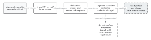
The finite-volume partition function generates response, Legendre transforms change controlled variables, and large-deviation rate functions encode phase weights only after the thermodynamic-limit order is declared. Solid connections show the primary relation; dashed outlines or arrows mark qualifications and failure boundaries. The diagram is schematic and not to scale.

The surrounding discussion supplies the relevant equations and checks in text form; the figure is a navigational summary.

Exercise

Let $M_V$ be the sum of $V$ independent spins taking $\pm1$ with equal probability. Find $\lambda(k)$ and the rate function.

Solution

$\langle e^{kM_V}\rangle=(\cosh k)^V$, so $\lambda(k)=\log\cosh k$. The stationary condition $m=\tanh k$ gives $k=\operatorname{arctanh}m$ and

$$I(m)=\frac{1+m}{2}\log(1+m) +\frac{1-m}{2}\log(1-m),$$

for $\lvert m\rvert\le1$, with the convention $I(0)=0$. Its curvature $I''(0)=1$ reproduces variance $1/V$ for the mean magnetization.

References

• Ellis, Richard S. Entropy, Large Deviations, and Statistical Mechanics. New York: Springer, 1985. doi:10.1007/978-1-4613-8533-2.
• Gärtner, Jürgen. “On Large Deviations from the Invariant Measure.” Theory of Probability & Its Applications 22, no. 1 (1977): 24–39. doi:10.1137/1122003.
• Touchette, Hugo. “The Large Deviation Approach to Statistical Mechanics.” Physics Reports 478, nos. 1–3 (2009): 1–69. doi:10.1016/j.physrep.2009.05.002; Open PDF.