Wigner Transformation and Gradient Expansion

The Wigner transform rewrites two-point functions in center coordinates $X=(x+y)/2$ and relative coordinates $s=x-y$. It does not make a system kinetic by itself. Local transport emerges only if derivatives with respect to $X$ are small compared with the inverse relative-time and relative-distance scales carried by the spectral and memory kernels.

Required background. Use the Kadanoff–Baym equations for the unreduced two-time dynamics and tempered distributions and Fourier calculus for distributional transforms.

Helpful background. Kadanoff–Baym reduction to kinetic theory continues from the first-order equations to collision terms and matching.

Wigner coordinates and finite-time qualification

For a bi-local kernel $A(x,y)$ define

$$A_W(X,p)=\int d^{d+1}s\,e^{ip\cdot s} A\!\left(X+\frac{s}{2},X-\frac{s}{2}\right).$$

If the initial time is finite, the relative-time integral is not over the whole real line: both arguments must remain later than $t_0$, so $|s^0|\le 2(X^0-t_0)$. Extending the limits to infinity discards preparation-edge terms and requires loss of sensitivity to the initial boundary. A finite window also convolves the true spectrum with the window transform, limiting frequency resolution by $\Delta\omega\gtrsim1/s^0_{\max}$.

For charged or non-Abelian fields, $A(x,y)$ at separated points is not gauge covariant without parallel transport. A gauge-covariant Wigner function inserts a Wilson line between the endpoints; expanding it produces field-strength terms. Replacing ordinary derivatives by covariant derivatives after performing a noncovariant transform does not recover the missing information.

The Moyal product

For the spacetime convolution $(A\circ B)(x,y)=\int dz\,A(x,z)B(z,y)$, the phase-space product introduced in Moyal 1949, §§ 3–4 is exactly

$$(A\circ B)_W =A_W\exp\!\left[ \frac{i}{2}\left( \overleftarrow{\partial}_X\!\cdot\!\overrightarrow{\partial}_p -\overleftarrow{\partial}_p\!\cdot\!\overrightarrow{\partial}_X \right)\right]B_W \equiv A_W\star B_W.$$

To first order,

$$A\star B=AB+\frac{i}{2}\{A,B\}_{\mathrm{PB}}+O(\partial_X^2), \qquad \{A,B\}_{\mathrm{PB}} =\partial_XA\cdot\partial_pB-\partial_pA\cdot\partial_XB.$$

The controlling ratios are problem-dependent: typical examples are $\ell_{\mathrm{micro}}/L_X$, $\tau_{\mathrm{corr}}/\tau_X$, or a background force over the momentum scale. A narrow spectral width can increase the correlation time and spoil the expansion even at weak coupling. Rapid phases and shell singularities also make nominally higher derivatives large.

Constraint and transport equations

The Wigner-transformed retarded Dyson equation has the schematic form

$$\big[p^2-M^2(X)-\Sigma_R(X,p)\big]\star G_R(X,p)=1.$$

Its real part provides a spectral or constraint equation; its imaginary part controls the width. The statistical Kadanoff–Baym equation can be organized into an anticommutator-like constraint and a commutator-like transport equation. At first gradient order the latter contains Poisson brackets such as

$$\{p^2-M^2-\operatorname{Re}\Sigma_R,F\}_{\mathrm{PB}} =\Sigma_\rho F-\Sigma_F\rho+\text{first-order backflow terms}.$$

Dropping the backflow terms, imposing $F\propto(1/2+f)\rho$, and replacing $\rho$ by an on-shell delta function are separate approximations. They require finite-width and gradient checks; none follows solely from performing the transform.

The right half of the hierarchy separates an exact change of variables from approximations. The Wigner transform itself is reversible when boundary information is retained; truncating the Moyal series and projecting onto a narrow shell are independent expansions.

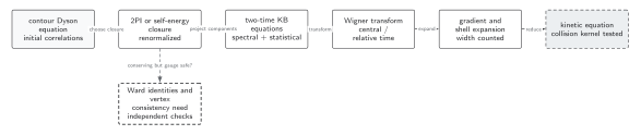
Central and relative coordinates reorganize the two-time equations without yet discarding information. A local kinetic equation appears only after a controlled gradient expansion, a justified spectral-width or shell treatment, and any memory approximation; finite initial time can also generate boundary terms. Each small parameter must be counted and tested separately. The diagram is schematic and not to scale.

The sections Wigner coordinates and finite-time qualification, The Moyal product, and Constraint and transport equations give the text and equation equivalent of the transform and expansion boxes.

Checked convolution example

Let $A(X,p)=a(X)$ and $B(X,p)=b(p)$. Then

$$A\star B=a(X)b(p)+\frac{i}{2}\partial_Xa\cdot\partial_pb+O(\partial_X^2).$$

For $a(X)=a_0e^{iq\cdot X}$, the expansion parameter acting on $b$ is $q\cdot\partial_pb$. If $b$ changes on a momentum scale $\Delta p$, control requires $|q|/\Delta p\ll1$. A sharply peaked $b$ can therefore invalidate the gradient expansion even when $a$ looks slowly varying in absolute units.

Failure tests

• Compare zeroth-, first-, and second-order Moyal terms on the actual solution rather than estimating derivatives from input scales alone.
• Increase the relative-time window and vary the window function; stable peak positions with unstable widths do not establish a resolved spectral width.
• Retain the finite-$t_0$ boundary once and verify that discarding it changes target observables below the stated error.
• In gauge theories, change path prescriptions consistently and test gauge-covariant constraints or Ward identities.
• Benchmark the reduced equations against the unreduced two-time evolution. The validation matrix records the required comparison.

Exercise

Show that the star commutator $A\star B-B\star A$ contains $i\{A,B\}_{\mathrm{PB}}$ at first order, while the star anticommutator has no first-order term for commuting scalar functions.

Solution

Expanding both products gives $A\star B=AB+(i/2)\{A,B\}_{\mathrm{PB}}+O(\partial_X^2)$ and $B\star A=BA-(i/2)\{A,B\}_{\mathrm{PB}}+O(\partial_X^2)$. For commuting scalar functions, subtraction yields $i\{A,B\}_{\mathrm{PB}}$ and addition yields $2AB+O(\partial_X^2)$.

Continue

Use spectral and statistical evolution to decide whether a quasiparticle occupation is meaningful, then compare any kinetic reduction with numerical two-time evolution.

References

• Botermans, W., and Malfliet, R. (1990). “Quantum Transport Theory of Nuclear Matter.” Physics Reports 198, 115–194. DOI.
• Moyal, J. E. (1949). “Quantum Mechanics as a Statistical Theory.” Mathematical Proceedings of the Cambridge Philosophical Society 45, 99–124. DOI.
• Wigner, E. (1932). “On the Quantum Correction for Thermodynamic Equilibrium.” Physical Review 40, 749–759. DOI.