Weak-Coupling Plasma Transport Coefficients

Weak-coupling transport coefficients are inverse relaxation rates of nearly conserved distortions. Their leading-order values follow from a linearized gauge-theory collision operator or, equivalently, from the narrow low-frequency structure required by Kubo formulas. The calculation is not a single cross section: screened elastic exchange, collinear number-changing processes, exact zero modes, and a controlled numerical inversion all matter.

Required background. Gauge-theory EKT supplies the collision operator, and sources, linear response, and Kubo formulas supplies the response definitions. Helpful background. Transport inverse problems and error budgets explains why a fitted coefficient is conditional on its model and covariance.

Linearized collision problem

Write a small departure from equilibrium as

$$f_a=f_a^{(0)} +f_a^{(0)}(1\pm f_a^{(0)})\,\chi_a.$$

An applied velocity gradient, electric field, or chemical-potential gradient produces a source $S$. Linearization gives

$$S=\mathcal C_{\rm lin}\chi .$$

With the equilibrium-weighted inner product, detailed balance makes the collision operator nonnegative:

$$(\chi,\mathcal C_{\rm lin}\chi)\ge0.$$

Its null space consists of exactly conserved quantities. The source must be orthogonal to those zero modes, or matching conditions must project them out. Otherwise the inverse does not exist. This mathematical fact is the kinetic expression of hydrodynamic conservation laws.

For shear flow, the tensor structure is

$$\chi_a(\mathbf p)=\chi_a(p) \left(\hat p_i\hat p_j-\frac13\delta_{ij}\right)\sigma_{ij},$$

and the solution determines

$$\eta=\frac{\beta}{10}\sum_a\nu_a \int\frac{d^3p}{(2\pi)^3} \frac{p^4}{E_p^2} f_a^{(0)}(1\pm f_a^{(0)})\,\chi_a(p),$$

with normalization conventions absorbed into $\chi_a$. Charge conductivity and diffusion use vector sources; bulk viscosity uses a scalar source orthogonal to energy conservation and is especially sensitive to conformal-symmetry breaking and number-changing processes.

Variational solution and bounds

Define

$$\mathcal Q[\chi]=(\chi,S)-\frac12(\chi,\mathcal C_{\rm lin}\chi).$$

The stationary condition is $\mathcal C_{\rm lin}\chi=S$, and at the maximum

$$\mathcal Q_{\max}=\frac12(S,\mathcal C_{\rm lin}^{-1}S).$$

Expanding $\chi$ in a finite basis converts the problem to a positive semidefinite matrix equation after zero modes are removed. Enlarging a nested basis gives a monotone sequence for the variational functional, a valuable convergence check. Arnold, Moore, and Yaffe used this framework to obtain complete leading-order shear viscosity in gauge theories Arnold, Moore, and Yaffe 2003, §§ 2–6.

The leading parametric behavior is

$$\eta\sim\frac{T^3}{g^4\ln(1/g)},\qquad D\sim\frac{1}{g^4T\ln(1/g)},\qquad \sigma_{\rm el}\sim\frac{T}{g^4\ln(1/g)}$$

up to charge factors and the fact that complete leading order changes both coefficients and the effective logarithm. These scalings express slow large-angle relaxation, not universal numerical formulas.

Momentum broadening and operator definitions

For a highly energetic parton, the transverse broadening parameter is often introduced as

$$\hat q_R=\frac{d}{dL}\langle p_\perp^2\rangle_R.$$

Beyond this mnemonic it must be defined by a lightlike or nearly lightlike Wilson-line correlator, with representation $R$, rapidity prescription, renormalization scheme, and kinematic cutoff specified. Its soft contribution can be matched to EQCD in suitable regimes Caron-Huot 2009, while hard momentum transfers and finite-energy corrections require separate treatment. A phenomenological “$\hat q$” inferred inside a shower model is conditional on that model’s splitting, recoil, medium, and hadronization choices.

Error budget and limits

A complete transport result reports:

• coupling and renormalization convention;
• screened $2\leftrightarrow2$ and LPM $1\leftrightarrow2$ kernels at the same order;
• collision-operator conservation and detailed-balance residuals;
• basis, momentum-grid, and integration convergence;
• separation-scale cancellation;
• truncation uncertainty, distinguished from numerical error;
• the domain in temperature, chemical potential, and anisotropy.

These fields align with the hot-gauge plasma validity table. Leading-order weak-coupling values are benchmarks; applying them at $g=O(1)$ is a phenomenological extrapolation. A small value of $\eta/s$ inferred from collision data cannot be compared directly to a weak-coupling $\eta$ without a common equation of state, definition, scale, and uncertainty model.

Transport coefficients occupy the near-equilibrium linear-response branch of the diagram and should not be identified with instability growth rates or hard-probe kernels.

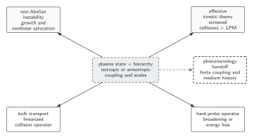
Bulk viscosity, shear viscosity, diffusion, and conductivity arise from source-dependent inversions of a linearized collision operator with its conserved zero modes removed. The instability branch applies to anisotropic states, while hard-probe coefficients sample different Wilson-line or collision kernels. The dashed phenomenology branch marks additional finite-coupling and medium-history uncertainty. The diagram is schematic and not to scale.

The text equivalent is to state the Kubo normalization or kinetic source, enforce Landau matching and conserved-mode constraints, solve with controlled screening and collinear kernels, and report numerical and coupling uncertainties. A coefficient inferred from collision data is not a direct measurement of the weak-coupling quantity without this matching.

Exercises

1. Variational stationarity. Vary $\mathcal Q[\chi]$ and show that its stationary point solves the linearized Boltzmann equation.

Solution

For an arbitrary $\delta\chi$ and self-adjoint $\mathcal C_{\rm lin}$, $\delta\mathcal Q=(\delta\chi,S-\mathcal C_{\rm lin}\chi)$. It vanishes for every allowed $\delta\chi$ exactly when $\mathcal C_{\rm lin}\chi=S$, after projection away from zero modes.

2. Einstein relation. If a conserved density has susceptibility $\chi_Q$ and constitutive law $\mathbf J=-D\nabla n+\sigma\mathbf E$, show that equilibrium thermodynamics implies $\sigma=\chi_QD$ in units where the charge is included in $\chi_Q$.

Solution

Write $\nabla n=\chi_Q\nabla\mu$. Electrochemical equilibrium requires the current to depend on $\nabla\mu-\mathbf E$, so $\mathbf J=-D\chi_Q\nabla\mu+\sigma\mathbf E$ vanishes when $\nabla\mu=\mathbf E$. Hence $\sigma=D\chi_Q$.

Continue to non-Abelian plasma instabilities for a competing anisotropic weak-coupling mechanism.

References

• Arnold, Peter, Guy D. Moore, and Laurence G. Yaffe. “Transport Coefficients in High Temperature Gauge Theories: (I) Leading-Log Results.” Journal of High Energy Physics 2000, no. 11 (2000): 001. DOI.
• Arnold, Peter, Guy D. Moore, and Laurence G. Yaffe. “Transport Coefficients in High Temperature Gauge Theories: (II) Beyond Leading Log.” Journal of High Energy Physics 2003, no. 5 (2003): 051. DOI.
• Caron-Huot, Simon. “O(g) Plasma Effects in Jet Quenching.” Physical Review D 79, no. 6 (2009): 065039. DOI.
• Jeon, Sangyong. “Hydrodynamic Transport Coefficients in Relativistic Scalar Field Theory.” Physical Review D 52, no. 6 (1995): 3591–3642. DOI.