Sources, Linear Response, and Kubo Formulae

A weak source produces a retarded response because the perturbation acts only at earlier times. With the convention $G^R=-i\theta\langle[\ ,\ ]\rangle$ and a Hamiltonian coupling $H_f=H_0-\int f_B B$, the physical linear kernel is $\mathcal R_{AB}=-G^R_{AB}$ plus local source contacts. A transport coefficient is then a specified low-frequency, low-momentum limit of this complete kernel—not of an unspecified two-point function.

Required background. Spurions, local counterterms, and symmetry response explains how observables are obtained by varying background fields and why local counterterms matter. Closed-time-path generating functionals supply normalized real-time source differentiation. Helpful background. Sources and nonlinear response extends the construction to multiple insertions.

Causal response from a Hamiltonian source

Let the equilibrium state of $H_0$ be perturbed by

$$H_f(t)=H_0-\int d^{d_s}x\,f_B(t,\mathbf x)B(t,\mathbf x).$$

To first order, interaction-picture evolution gives

$$\begin{aligned} \delta\langle A(t,\mathbf x)\rangle &=-i\int_{-\infty}^{t}dt'\,\langle[A(t,\mathbf x),H_f(t')-H_0]\rangle_0\\ &=\int d^{d_s+1}x'\;i\theta(t-t') \langle[A(x),B(x')]\rangle_0 f_B(x'). \end{aligned}$$

Thus

$$\mathcal R^{\mathrm{nonlocal}}_{AB}(x-x') =\frac{\delta\langle A(x)\rangle}{\delta f_B(x')} =i\theta(t-t')\langle[A(x),B(x')]\rangle =-G^R_{AB}(x-x').$$

If $A$ itself depends on the source, differentiation also produces an equal-time local term,

$$\mathcal R_{AB}(x,x')=-G^R_{AB}(x,x') +C_{AB}(x,x'), \qquad C_{AB}=\left\langle\frac{\delta A_f(x)}{\delta f_B(x')}\right\rangle_{f=0}.$$

Diamagnetic current response and pressure seagulls are examples. Their sign and normalization follow from the source functional; they cannot be restored reliably after computing only the commutator. Kubo’s original construction and modern thermal-field-theory treatments derive the same causal kernel Kubo 1957, §§2–3 Kovtun 2012, §§2.2–2.3, Open PDF.

Spectral representation and the dissipative slope

For a Hermitian bosonic operator in a stationary state,

$$G^R_{AA}(z,\mathbf k) =\int_{-\infty}^{\infty}\frac{d\omega'}{2\pi} \frac{\rho_{AA}(\omega',\mathbf k)}{z-\omega'}, \qquad \operatorname{Im}z>0,$$

so that $\rho_{AA}=-2\operatorname{Im}G^R_{AA}$ on the real axis. In a passive equilibrium system, $\rho_{AA}(\omega,\mathbf k)/\omega\ge0$ for the diagonal channel. Consequently a dissipative coefficient extracted as

$$\lambda =-\lim_{\omega\to0^+}\frac{1}{\omega} \operatorname{Im}G^R_{\mathcal O\mathcal O}(\omega,\mathbf0) =\lim_{\omega\to0^+}\frac{\rho_{\mathcal O\mathcal O}(\omega,\mathbf0)}{2\omega}$$

is nonnegative once the operator normalization and tensor projector are fixed. Off-diagonal channels instead obey matrix positivity and Onsager–Casimir relations; an individual cross coefficient need not be positive.

Static response is a different limit. For a source held constant in time and space,

$$\chi_{AB}=\lim_{\mathbf k\to\mathbf0} \lim_{\omega\to0}\mathcal R_{AB}(\omega,\mathbf k),$$

whereas a homogeneous transport measurement normally takes $\mathbf k=0$ first and then examines $\omega\to0$. Hydrodynamic poles make the two paths unequal. The equilibrium state, tensor sector, and quantities held fixed must accompany either formula.

Conductivity as a complete response

Couple a spatial vector potential by $H[A]=H_0-\int J^iA_i+O(A^2)$. In temporal gauge and at zero momentum, $E_i(\omega)=i\omega A_i(\omega)$. Define the complete homogeneous current kernel

$$K^{ij}(\omega)=\frac{\delta\langle J^i\rangle}{\delta A_j} =-G_R^{J^iJ^j}(\omega,\mathbf0)+C^{ij}.$$

Then

$$\sigma^{ij}(\omega)=\frac{K^{ij}(\omega)}{i(\omega+i0^+)}.$$

Gauge invariance fixes the cancellation between the zero-frequency paramagnetic correlator and the diamagnetic contact in a normal phase. If momentum or another exactly conserved operator overlaps with $J^i$, $\operatorname{Re}\sigma$ also contains a delta function; the regular dc conductivity is not obtained by silently discarding it. The same source logic applied to a metric perturbation yields the shear and bulk stress Kubo formulae, including pressure contacts Hartnoll, Lucas, and Sachdev 2018, §§2.1–2.2, Open PDF.

Tensor projections and normalization

For an isotropic medium, a spatial current correlator splits into longitudinal and transverse projectors,

$$G_R^{ij}=P_L^{ij}G_L+P_T^{ij}G_T, \qquad P_L^{ij}=\frac{k^ik^j}{k^2}, \qquad P_T^{ij}=\delta^{ij}-P_L^{ij}.$$

At $k=0$ rotational symmetry gives a scalar conductivity only after division by the number of averaged directions. Stress response likewise requires a normalized rank-four projector. Writing merely “the $T^{ij}$ correlator” leaves factors of two and $d_s$ ambiguous. Improvement terms can also change local contacts while leaving separated-point conservation laws intact.

Standard many-body derivations of current contacts, spectral response, and conductivity normalizations are collected in Mahan 2000, chs. 3–4.

Transport-extraction covariance reference

Every row is a reproducibility record, not a promise that the named coefficient is identifiable. “Resolution” means the averaging kernel or smallest distinguishable spectral scale, not merely the sampling interval.

Claim or channel	Operator, source, and response convention	Contacts, subtractions, and conserved overlap	Limit order and spectral constraint	Inverse method, prior, covariance, resolution, and fit window	Continuum, volume, cross-check, and evidence date
Static susceptibility	State $A,B$, the sign in $H_f$, and $\mathcal R=-G_R+C$	Equal-time contact; thermodynamic variables held fixed	$\omega\to0$ before $k\to0$; compare the thermodynamic Hessian	Usually direct; publish full covariance and finite-difference window	Extrapolate regulator and volume; Ward/Hessian check; date the inputs
Electrical conductivity	Current normalization and background gauge field	Diamagnetic term, magnetization current, momentum Drude weight	$k=0$, then $\omega\to0$; charge sum rule	State real-time fit or continuation prior, covariance, low-frequency resolution, and window	Continuum/thermodynamic limits; gauge Ward identity and synthetic peak recovery; date
Thermal or Hall transport	Heat-current definition and metric or thermal source	Energy magnetization, electric-current mixing, open-circuit subtraction	State longitudinal/transverse sector and dc path	Publish joint covariance of thermoelectric channels and resolution of antisymmetric pieces	Boundary/volume prescription; Onsager–Casimir and equilibrium-current checks; date
Diffusion eigenvalue	Density basis, chemical-potential sources, $\Sigma$, and $\chi$	Project exact conserved zero modes; retain matrix structure	Hydrodynamic pole at small nonzero $k$ before extrapolating $k\to0$	Correlated pole fit or generalized eigenproblem; prior and $k$ window	Volume and discretization scaling; Einstein relation and mode-residue check; date
Shear viscosity	Normalized traceless stress projector and metric source	Pressure/seagull contact and any elastic delta weight	$k=0$, $\omega\to0^+$; stress sum rules	State spectral ansatz or real-time window, covariance, slope resolution, and UV matching	Continuum/volume limits; tensor Ward identity and benchmark recovery; date
Bulk viscosity	Thermodynamically projected scalar stress	Subtract energy and charge densities; isolate sound and critical modes	Specify $k=0$ transport limit and scalar-channel sum rule	Jointly vary slow-mode and UV models; publish covariance and resolvable width	Check conformal limit, finite size, regulator, and Hydro+ sensitivity; date
Memory-matrix rate	Slow basis, Kubo–Mori product, and operator normalization	Include every exactly conserved overlap and incoherent remainder	Weak-breaking limit before dc limit, with projected spectral weight	State truncation as model choice; propagate susceptibility and kernel covariance	Enlarge the slow basis; compare kinetic/hydrodynamic limits; date
Euclidean spectral extraction	Euclidean operator normalization and thermal kernel	Remove contacts and known UV pieces before continuation	Enforce only justified positivity, moments, and sum rules	Publish likelihood covariance, priors/ansätze, resolution matrix, validation split, and windows	Continuum/volume extrapolation; mock-data recovery, posterior prediction, and dated inputs

The contact and magnetization page explains the second column of corrections; the inverse-problem page explains why the last two columns determine the strength of the final claim.

Checks and limitations

Three checks are independent of a microscopic model. First, the retarded function must be analytic for $\operatorname{Im}\omega>0$. Second, Ward identities must hold for the complete response, contacts included. Third, diagonal dissipative spectral weight must have the sign required by passivity. These do not establish that a low-frequency slope is numerically resolved.

A hydrodynamic formula controls only frequencies and momenta below the first omitted relaxation scale. A Euclidean correlator averages over frequency and can be almost unchanged while the dc slope varies greatly. A successful fit therefore licenses only those combinations stable under covariance propagation, resolution tests, and defensible variations of the forward model.

The first three boxes below condense the definition stage developed on this page. Inspect the order: normalize the operator and source, differentiate to obtain the complete response, and only then subtract contacts and specify the Kubo limit.

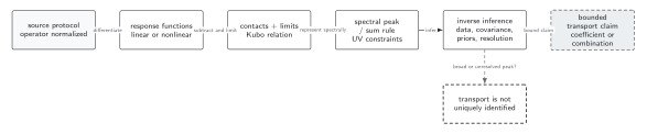
A transport definition begins with an operator normalized against its physical source. Functional differentiation fixes the response sign and local contacts; the declared frequency–momentum path fixes the Kubo observable. Spectral constraints and inverse inference enter only afterward. The diagram is a schematic logic chain, not a claim that every dataset determines the final coefficient.

In text: state $H_f$, compute $\mathcal R=-G_R+C$ in the site’s convention, include diamagnetic or pressure contacts, normalize the tensor projector, and declare the order of limits. The remaining boxes ask whether spectral information and data resolution support a coefficient, only a combination, or no unique transport claim.

Exercise: a single relaxation pole

Suppose a physical response is

$$\mathcal R(\omega)=\chi\frac{\Gamma}{\Gamma-i\omega}, \qquad \chi>0,\quad\Gamma>0,$$

with no contact term. Find $G_R$, its spectral function, and the static susceptibility. Check analyticity and positivity.

Solution

Because $\mathcal R=-G_R$,

$$G_R(\omega)=-\chi\frac{\Gamma}{\Gamma-i\omega}.$$

Its only pole is at $\omega=-i\Gamma$, in the lower half-plane, so it is retarded. Moreover

$$\rho(\omega)=-2\operatorname{Im}G_R(\omega) =\frac{2\chi\Gamma\omega}{\Gamma^2+\omega^2},$$

and $\rho/\omega\ge0$. Finally $\mathcal R(0)=\chi$, as required. This check would fail in all three ways if the retarded sign or pole prescription were reversed.

References

• Hartnoll, Sean A., Andrew Lucas, and Subir Sachdev. 2018. Holographic Quantum Matter. Cambridge, MA: MIT Press. Publisher. Open PDF.
• Kovtun, Pavel. 2012. “Lectures on Hydrodynamic Fluctuations in Relativistic Theories.” Journal of Physics A: Mathematical and Theoretical 45 (47): 473001. DOI. Open PDF.
• Kubo, Ryogo. 1957. “Statistical-Mechanical Theory of Irreversible Processes. I. General Theory and Simple Applications to Magnetic and Conduction Problems.” Journal of the Physical Society of Japan 12 (6): 570–586. DOI.
• Mahan, Gerald D. 2000. Many-Particle Physics. 3rd ed. New York: Kluwer Academic/Plenum. DOI.

Contact Terms, Magnetization Currents, and Order of Limits now determines which local and circulating pieces enter a concrete experiment. Nonlinear Response and Higher-Order Kubo Relations extends the causal derivation beyond first order.