

The H-Theorem and Kinetic Entropy Production
The kinetic H-theorem proves nonnegative entropy production for positive distributions evolved by a microreversible, Markovian collision operator with factorized incoming correlations. It does not prove growth of the fine-grained von Neumann entropy of a closed quantum state, which remains constant under unitary evolution.
Required background. Use collision kernels, conservation, and detailed balance.
Helpful background. Onsager reciprocity and entropy production connects the near-equilibrium collision form to macroscopic transport.
Quantum kinetic entropy
Section titled “Quantum kinetic entropy”With for bosons and for fermions, use the quantum-statistical entropy underlying Uehling and Uhlenbeck 1933, pp. 554–557:
This requires for bosons and for fermions. Differentiating and using the kinetic equation gives
apart from boundary and mean-field terms whose entropy flux must be included.
For one reaction, define
After symmetrizing the four legs with the same positive transition weight,
because for positive . The proof fails if the transition weight is negative, inverse processes are missing, or gain and loss use inconsistent approximations.
Zero production and equilibrium family
Section titled “Zero production and equilibrium family”Entropy production vanishes when for every allowed reaction. Hence
must be a collision invariant: a linear combination of and charges conserved by the complete reaction network. This gives
For a homogeneous equilibrium, and . Extra chemical potentials disappear when number-changing reactions violate the corresponding charges. If the reaction graph is disconnected, additional stationary families can occur; ergodicity is a separate requirement.
The hierarchy sends a collision kernel to an “H theorem / relaxation modes” box only after conservation and detailed balance have been checked. That arrow is conditional: conservation alone does not give monotonic entropy production.
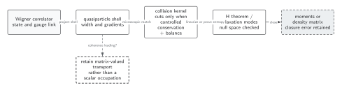
Entropy monotonicity follows for the stated positive gain–loss structure with the correct Bose or Fermi factors, microreversibility, and detailed balance. It is not guaranteed by an arbitrary conserving kernel, by a finite moment truncation, or by matrix-valued coherent evolution. The microscopic-matching step may use cuts in a controlled weak-coupling construction, but cuts are not a premise of every H theorem. The same collision operator may instead be assessed through its null space and relaxation spectrum. The diagram is schematic and not to scale.
The sections Quantum kinetic entropy, Zero production and equilibrium family, and Where monotonicity enters give the text and equation equivalent of the entropy branch and its hypotheses.
Where monotonicity enters
Section titled “Where monotonicity enters”The BBGKY or Kadanoff–Baym hierarchy contains correlations and memory. Molecular chaos replaces incoming pair correlations by products of one-particle distributions, and the Markov limit selects a retarded collision history. These steps discard information from the reduced state. The entropy above measures that coarse-grained description.
Coherent matrix distributions require a different entropy functional and a collision generator that preserves positivity. Off-shell spectral functions and non-Markovian kernels can make entropy production nonlocal in time and not sign definite instantaneously. Boundary flux can reduce entropy inside a finite region even when total production plus flux is nonnegative.
Checked classical limit
Section titled “Checked classical limit”For , the entropy density becomes
The reaction factor reduces to , , reproducing Boltzmann’s classical proof. An equilibrium Maxwell–Boltzmann form makes a linear combination of collision invariants.
Failure tests
Section titled “Failure tests”- Monitor bosonic positivity and the fermionic upper bound.
- Verify microreversibility and include inverse and number-changing reactions.
- Preserve collision invariants in the discretized operator.
- Account for boundary entropy flux and external work.
- Compare with a correlation-sensitive or two-time description when memory or coherence is appreciable.
- Never identify kinetic entropy with fine-grained quantum entropy without a coarse-graining statement.
Exercise
Section titled “Exercise”Prove for positive .
Solution
The logarithm is strictly increasing, so and have the same sign. Their product is nonnegative and vanishes only at .
Continue
Section titled “Continue”Use entropy production as one diagnostic—not the only one—in moment closures and kinetic validity.
References
Section titled “References”- Boltzmann, L. (1872). “Further Studies on the Thermal Equilibrium of Gas Molecules.” Sitzungsberichte der Kaiserlichen Akademie der Wissenschaften 66, 275–370. English translation.
- Uehling, E. A., and Uhlenbeck, G. E. (1933). “Transport Phenomena in Einstein–Bose and Fermi–Dirac Gases. I.” Physical Review 43, 552–561. DOI.
Original QFT.org content:CC BY 4.0, unless an item supplies different terms. Third-party material retains its own terms.