Euclidean and Real-Time Access at Finite Density

No single method accesses every finite-density observable. Taylor and imaginary-chemical-potential approaches are controlled inside an analyticity domain; canonical sectors and reweighting face volume-dependent overlap; complex Langevin and contour deformations require method-specific correctness tests; real-time formulations inherit oscillatory weights; low-density EFTs are reliable only within their power counting. The correct choice follows from the observable, density regime, analytic structure, volume, target precision, and a benchmark that can expose failure.

The complex-weight, overlap, and analytic-access limitations at baryon density are reviewed by de Forcrand 2010, §§ 2–5.

Required background. Silver Blaze Behavior, Thresholds, and Density Instabilities fixes the physical singularities that bound continuation. Helpful background. Chemical Potential on the Euclidean Lattice owns regulator-specific lattice constructions. Noisy Spectral Reconstruction as an Inverse Problem supplies the separate Euclidean-to-real-time claim ceiling.

Why the weight becomes complex

At real chemical potential, a Euclidean fermion determinant generally obeys

$$\det M(\mu)^*=\det M(-\mu^*)$$

rather than $\det M(\mu)^*=\det M(\mu)$. Importance sampling with a positive probability measure therefore fails. Phase reweighting writes

$$\langle\mathcal O\rangle =\frac{\langle\mathcal Oe^{i\theta}\rangle_{\mathrm{pq}}} {\langle e^{i\theta}\rangle_{\mathrm{pq}}},$$

but the average phase can scale as

$$\langle e^{i\theta}\rangle_{\mathrm{pq}} \sim e^{-V\Delta f/T}.$$

An exponentially small denominator is an overlap problem as well as a noisy phase. It can demand exponentially many samples; calling it merely “slow computation” understates the information loss.

Access matrix

Method	Controlled input	Principal barrier	Required negative control	Claim ceiling
Taylor expansion at $\mu=0$	derivatives/cumulants at zero density	nearest complex singularity and coefficient noise	recover a known singularity from held-out orders	within demonstrated convergence or resummation domain
Imaginary $\mu$	positive or more tractable unitary holonomy	analytic continuation and phase boundaries	vary ansatz/order and test known periodicity	real-$\mu$ result inside verified analytic domain
Reweighting	ensemble at reference parameters	exponentially poor overlap	independent ensembles bracketing target	only where effective sample size and tails are controlled
Canonical sectors	Fourier projection in imaginary $\mu$	oscillatory projection and large-charge resolution	reconstruct the grand partition function	resolved charge sectors at declared volume
Complex Langevin	complexified stochastic process	wrong stationary limit from poles or broad tails	solvable benchmark, identities, excursion/tail diagnostics	conditional on correctness criteria and cross-method agreement
Lefschetz/thimble methods	contour decomposition	many relevant thimbles, residual phase, Stokes jumps	reproduce original contour in a benchmark	conditional finite-volume integral with decomposition error
Real-time methods	direct contour evolution	oscillatory phase, entanglement or memory growth	unitary and conservation benchmarks	bounded time/volume and observable-specific result
Low-density EFT	scale separation and matched couplings	breakdown near new thresholds or dense phases	order-by-order residual and alternative matching	observables within stated power counting

The method names do not establish their domain. Each row is an inference contract to be validated on the target observable.

Analytic expansions and their limits

For pressure,

$$\frac{p(T,\mu)}{T^d} =\sum_{n=0}^{\infty}c_n(T) \left(\frac{\mu}{T}\right)^n.$$

Charge-conjugation symmetry can remove odd terms, but the radius of convergence is set by the nearest singularity in the complex $\mu$ plane, not necessarily a real critical point. Finite order cannot uniquely distinguish a real-axis singularity from a complex pair. Ratio estimators, Padé approximants, and conformal maps add assumptions whose stability must be tested against synthetic functions with known singularities.

Imaginary-$\mu$ data exploit a unitary holonomy and exact periodicity. Continuing a polynomial fit past a Roberge–Weiss or other nonanalytic boundary is invalid even if the fit residual remains small.

Complexified methods are not automatically exact

Complex Langevin can be correct when the complexified distribution decays sufficiently and integrations by parts receive no boundary contribution; meromorphic drifts and excursions can violate those conditions. Thimble decompositions preserve the integral only when all relevant cycles, intersection numbers, residual phases, and Stokes changes are handled. Neither method has a universal “sign problem solved” status.

Benchmark-first decision rule

Before entering an unresolved regime, choose a benchmark sharing the target’s determinant zeros, volume scaling, observable, and threshold structure. Blind the known answer if possible. Require:

• agreement among at least two independent routes in their overlap;
• correct Silver Blaze and onset behavior;
• volume and continuum trends;
• effective sample size or complex-distribution tail diagnostics;
• injected failure cases that the method rejects;
• uncertainty including truncation, continuation, and model choice; and
• a stopping rule before extrapolating past evidence.

Dense-QCD conclusions require the dedicated evidence boundaries in Chapter 18; this page supplies only the durable method logic.

The schematic below organizes the relationships used on this page. Inspect it with this question in mind: What can different finite-density access methods establish?

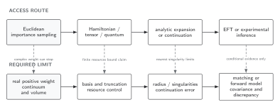
Euclidean, Hamiltonian, analytic, EFT, and experimental routes have different sign, overlap, continuation, volume, and model assumptions, so each supports a different ceiling on finite-density claims. The method columns are alternatives rather than stages of a universal pipeline; horizontal arrows organize cross-method comparison. Dashed marks show qualifications and failure boundaries. The diagram is schematic and not to scale.

The surrounding discussion supplies the relevant equations and checks in text form; the figure is a navigational summary.

Exercise

Why can small Taylor coefficients through order $(\mu/T)^8$ fail to establish a large radius of convergence?

Solution

A finite prefix can be reproduced by functions with very different higher-order coefficients and singularities. A nearby complex-conjugate pair can cause cancellations or oscillatory ratios, and coefficient uncertainty is amplified in high-order estimators. One needs stability across orders, analytic constraints, synthetic counterexamples, and ideally overlap with another method; eight small coefficients alone provide no rigorous lower bound.

References

• Aarts, Gert. “Introductory Lectures on Lattice QCD at Nonzero Baryon Number.” Journal of Physics: Conference Series 706 (2016): 022004. doi:10.1088/1742-6596/706/2/022004; Open PDF.
• de Forcrand, Philippe. “Simulating QCD at Finite Density.” Proceedings of Science LAT2009 (2010): 010. doi:10.22323/1.091.0010; Open PDF.
• Troyer, Matthias, and Uwe-Jens Wiese. “Computational Complexity and Fundamental Limitations to Fermionic Quantum Monte Carlo Simulations.” Physical Review Letters 94 (2005): 170201. doi:10.1103/PhysRevLett.94.170201.