Chemical Potential on the Euclidean Lattice

A chemical potential for a conserved charge is an imaginary temporal gauge field: on a Euclidean lattice it multiplies forward and backward temporal hops by reciprocal fugacity factors. This prescription reproduces $H-\mu Q$ without the spurious power divergences generated by adding a naive local number-density term. It also exposes precisely why a real baryon chemical potential usually destroys determinant positivity.

Required background. Fermion determinants, Pfaffians, and measure positivity supplies Grassmann integration and determinant symmetries. Euclidean correlators and Schwinger functions supplies the thermal path integral and antiperiodic fermion boundary condition.

Helpful background. In–out versus in–in expectation values clarifies why the equilibrium partition function here is not a real-time preparation protocol.

Temporal links and the conserved charge

Convention and regulator card. The lattice spacing is $a$, Euclidean time has $N_\tau$ sites and $T=(aN_\tau)^{-1}$, $\gamma_\nu^\dagger=\gamma_\nu$, and a fermion of charge $q$ has real chemical potential $\mu$. The link $U_4(x)$ transports from $x$ to $x+\hat4$. With the Wilson convention below, the continuum operator is $\gamma_\nu D_\nu+m-\mu q\gamma_4$. Reversing the definition of $Q$ or link orientation reverses both fugacity exponents; mixing conventions does not.

The grand-canonical trace is

$$Z(\beta,\mu)=\operatorname{Tr}\exp[-\beta(H-\mu Q)].$$

Divide Euclidean time into slices. Between adjacent slices, a state of charge $q$ acquires $e^{a\mu q}$ in the forward direction. Gauge covariance then requires the temporal link and fugacity to occur together. For Wilson fermions one convenient dimensionless matrix is

$$\begin{aligned} D_{xy}(\mu)={}&\delta_{xy} -\kappa\sum_{j=1}^{3}\left[(1-\gamma_j)U_j(x)\delta_{x+\hat j,y} +(1+\gamma_j)U_j^\dagger(x-\hat j)\delta_{x-\hat j,y}\right]\\ &-\kappa\left[e^{a\mu q}(1-\gamma_4)U_4(x)\delta_{x+\hat4,y} +e^{-a\mu q}(1+\gamma_4)U_4^\dagger(x-\hat4)\delta_{x-\hat4,y}\right]. \end{aligned}$$

This exponential prescription was introduced to avoid the quadratic divergence caused by a naive linear lattice insertion Hasenfratz and Karsch 1983, pp. 308–310. Expanding the temporal terms at fixed physical $\mu$,

$$e^{\pm a\mu q}=1\pm a\mu q+O(a^2),$$

and Taylor-expanding the neighboring fields and links gives

$$a^{-1}D(\mu)=\gamma_\nu D_\nu+m-\mu q\gamma_4+O(a),$$

after the usual Wilson mass normalization. The reciprocal factors are essential: they couple to oriented temporal propagation and preserve the lattice interpretation of $μ$ as a constant Abelian temporal connection.

Boundary twist and winding number

The same physics may be moved from the bulk links to the thermal boundary. In the continuum temporal term,

$$\bar\psi(\partial_\tau-\mu q)\psi,$$

set $\psi(\tau)=e^{\mu q\tau}\chi(\tau)$ and $\bar\psi(\tau)=e^{-\mu q\tau}\bar\chi(\tau)$. The bulk $μ$ disappears, but antiperiodicity becomes

$$\chi(\beta)=-e^{-\beta\mu q}\chi(0), \qquad \bar\chi(\beta)=-e^{\beta\mu q}\bar\chi(0).$$

On the lattice, a corresponding nonunitary field redefinition cancels $e^{\pm a\mu q}$ on all temporal links except the closing link. A closed worldline winding $W$ times around Euclidean time therefore carries $e^{\beta\mu qW}$. Local contractible loops contain equally many forward and backward temporal steps, so their fugacity factors cancel. This winding interpretation is the bridge to worldline and dual formulations.

For imaginary chemical potential, $μ=i\mu_I$, the boundary factor is a phase. Its periodicity can be enlarged or reduced by gauge-center transformations in specific gauge theories; any such periodicity must be derived from the theory’s charges and boundary conditions, not assumed from the generic twist above.

Determinant conjugation and positivity

At zero chemical potential the Wilson operator obeys $γ5$-Hermiticity. The temporal factors generalize it to

$$D(\mu)^\dagger=\gamma_5D(-\mu^*)\gamma_5.$$

Taking determinants gives

$$[\det D(\mu)]^*=\det D(-\mu^*).$$

Three cases must be distinguished.

• For real baryon chemical potential, $-\mu^*=-\mu$. No symmetry forces $\det D(\mu)$ at a fixed gauge field to be real, so importance sampling by that determinant generally fails.
• For imaginary $μ=i\mu_I$, one has $-\mu^*=\mu$. The determinant is real; an even number of degenerate flavors gives $[\det D(i\mu_I)]^{N_f}\ge0$, apart from any separate rooting or Pfaffian issue.
• For two flavors with opposite real chemical potentials, $\det D(\mu)\det D(-\mu)=|\det D(\mu)|^2\ge0$. This is the familiar isospin-type pairing, not the same ensemble as equal-sign baryon chemical potential.

These are configuration-wise statements. A real partition function obtained only after charge-conjugate configurations cancel does not create a nonnegative sampling measure.

Derivatives at zero density

Let $M(\mu)=D(\mu)$ and $W(\mu)=e^{-S_g}\det M(\mu)^{N_f}$. The elementary identity

$$\partial_\mu\log\det M=\operatorname{Tr}(M^{-1}M')$$

gives the charge-density estimator. For an observable $O$ that may itself depend on $μ$,

$$\partial_\mu\langle O\rangle =\langle O'\rangle +\operatorname{Cov}\!\left(O,N_f\operatorname{Tr}M^{-1}M'\right).$$

The second derivative contains

$$\partial_\mu^2\log\det M =\operatorname{Tr}\!\left(M^{-1}M''-M^{-1}M'M^{-1}M'\right),$$

plus covariance terms from differentiating the ensemble. Charge conjugation often makes odd derivatives of charge-even observables vanish at $μ=0$; that is a symmetry check, not permission to omit the noisy disconnected contributions at even order.

Exact one-angle benchmark

For $\beta_0=1$ and $h=0.2$, define

$$w(\theta;\mu)=e^{\beta_0\cos\theta} \bigl(1+he^{\mu+i\theta}\bigr) \bigl(1+he^{-\mu-i\theta}\bigr).$$

Expansion into Fourier modes gives

$$w=e^{\beta_0\cos\theta} \left[1+h^2+2h\cosh\mu\cos\theta +2ih\sinh\mu\sin\theta\right].$$

Using $\int_{-\pi}^{\pi}e^{\beta_0\cos\theta}\cos(n\theta)d\theta=2\pi I_n(\beta_0)$ and oddness of the sine term,

$$Z_1(\mu)=2\pi\left[(1+h^2)I_0(\beta_0) +2h\cosh\mu\,I_1(\beta_0)\right].$$

This benchmark tests four independent facts: $Z_1$ is even in real $μ$; $Z_1(i\mu_I)$ is obtained by $\cosh\mu\to\cos\mu_I$; the integrand is complex for generic real $μ$; and its imaginary part integrates to zero. A code that silently discards the imaginary integrand can reproduce $Z_1$ here because of parity while giving wrong values for phase-sensitive observables—an intentional adversarial test.

Limits of the construction

Chemical potential must couple to an exactly conserved lattice charge if the transfer-matrix interpretation is to remain exact at finite $a$. A local density operator that differs by cutoff terms can have the right formal continuum dimension yet introduce wrong ultraviolet behavior. Likewise, inserting $e^{a\mu}$ into spatial links, using the same exponent in both temporal directions, or treating $μ a$ as fixed during a continuum extrapolation changes the target theory.

The Silver Blaze phenomenon is not a claim that the determinant is $μ$-independent below onset. At low temperature, bulk observables may remain density independent over a range of real $μ$ even though individual determinants vary strongly; the constancy is produced by cancellations. The onset threshold depends on the charge convention and the lightest state per unit charge, and finite $T$, finite volume, discretization, and unphysical quark masses qualify the statement.

The severity map below places determinant complexity in a broader diagnostic structure. Follow the phase branch only after naming the sampling measure and observable; overlap, representation cost, and worst-case complexity are related questions but not synonyms for a small average phase.

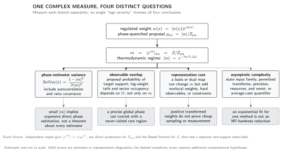
The sign problem has distinct diagnostics. The average phase fixes direct phase-estimator signal-to-noise and may scale as $e^{-\beta_TV_s\Delta f}$; overlap depends on the target observable and proposal measure; a variable change can trade phase for nonlocality or hard observables; and worst-case complexity requires a separately specified problem family. The map is schematic, not a quantitative performance comparison.

Observable-level validation checklist

• Verify $D(\mu)^\dagger=\gamma_5D(-\mu^*)\gamma_5$ numerically on representative gauge fields and check the paired-flavor positivity case separately.
• Recover the known free dispersion or number density as $a\to0$ at fixed physical $T$ and $μ$; do not hold $a\mu$ fixed.
• Check $μ=0$ derivatives against finite differences and symmetry-forbidden odd coefficients against zero.
• Compare bulk-link and boundary-twist implementations on the same finite lattice.
• Evaluate both $Z_1$ and at least one phase-sensitive observable in the one-angle fixture; parity cancellation alone is not enough.

Common pitfalls

A real partition function is not a positive measure. Charge conjugation can make $Z$ real only after integration. Importance sampling requires a nonnegative weight configuration by configuration.

Imaginary density is not real density with a harmless substitution. Analytic continuation is valid only within a common analytic domain and must respect periodicities and singularities; the continuation page gives that contract.

Exercises

1. Opposite chemical potentials

Show that two degenerate flavors with chemical potentials $μ$ and $-\mu$ have a nonnegative determinant product.

Solution

For real $μ$, determinant conjugation gives $[\det D(\mu)]^*=\det D(-\mu)$. Therefore

$$\det D(\mu)\det D(-\mu)=|\det D(\mu)|^2\ge0.$$

This assumes identical masses and lattice operators. It describes opposite charge chemical potentials; replacing it by equal-sign $μ$ changes the ensemble.

2. Number density in the exact fixture

Compute $n_1(\mu)=\partial_\mu\log Z_1(\mu)$ and check its value at $μ=0$.

Solution

Differentiating the exact expression gives

$$n_1(\mu)= \frac{2hI_1(\beta_0)\sinh\mu} {(1+h^2)I_0(\beta_0)+2hI_1(\beta_0)\cosh\mu}.$$

It is odd in $μ$ and vanishes at zero, as charge conjugation requires.

Learning outcomes

After working this page, you should be able to:

• Starting from a chosen temporal-link orientation, derive the $e^{\pm a\mu q}$ Wilson hops, their boundary twist, and the continuum term $-\mu q\bar\psi\gamma_4\psi$.
• Given a determinant relation and flavor assignment, decide whether the finite-density measure is complex, real with fluctuating sign, or nonnegative, and verify the decision on an explicit matrix.

Handoff

The operator has now been defined; anatomy and severity turns its complex phase into measurable signal-to-noise and overlap diagnostics. Canonical and fugacity methods later invert the winding-number expansion.

References

• Hasenfratz, Peter, and Frithjof Karsch. “Chemical Potential on the Lattice.” Physics Letters B 125 (1983): 308–310. doi:10.1016/0370-2693(83)91290-X.