Estimators, Covariance, and Resampling

Lattice observables are usually vectors of correlated means transformed through ratios, fits, scales, and renormalization factors. Reliable uncertainty requires the joint covariance and the correct independent unit—often a block of Markov history or an independent stream. Resampling individual measurements after their order has been discarded produces precise-looking but incorrect errors.

Required background. Markov-chain sampling defines the realized chain, and probabilistic limit theorems define the large-sample approximations.

Helpful background. Autocorrelation times determine a defensible block or replica unit.

Joint estimators and the delta method

Local statistical convention and regime. Inputs are ordered post-cut streams, and one resampling unit is a whole block or independent stream chosen from the slowest material influence direction. Each configuration contributes one joint measurement vector; components such as timeslices, numerator and denominator, scale, and matching factors are never resampled as independent observations when they share data. The full nonlinear estimator and any covariance regularization are recomputed inside every resample.

Let $\widehat{\boldsymbol\theta}$ estimate a vector $\boldsymbol\theta$ with covariance $\Sigma$. For a differentiable derived quantity $f$,

$$\operatorname{var}f(\widehat{\boldsymbol\theta}) \simeq \nabla f^T\Sigma\nabla f.$$

For a ratio $R=A/B$,

$$\operatorname{var}(R)\simeq \frac{\operatorname{var}(A)}{B^2} +\frac{A^2\operatorname{var}(B)}{B^4} -2\frac{A\operatorname{cov}(A,B)}{B^3}.$$

The covariance term can dominate. If numerator and denominator share configurations, omitting it is not conservative in a predictable direction.

Nonlinearity also induces $O(1/N)$ bias. A second-order expansion gives

$$\mathbb E[f(\widehat{\boldsymbol\theta})]-f(\boldsymbol\theta) \simeq\frac12\operatorname{tr}(H_f\Sigma),$$

where $H_f$ is the Hessian. Jackknife bias estimates or synthetic closure tests are useful when this is material.

Blocking before resampling

Partition each ordered stream into blocks long compared with relevant autocorrelation times and form block summaries. Blocks must not cross independent stream boundaries or parameter changes. Increase the block length until estimated uncertainty stabilizes while retaining enough blocks to estimate covariance; Geyer 1992, pp. 473–483 discusses this dependence-aware MCMC error problem.

For $N_b$ approximately independent blocks and estimator $\widehat\theta$, the delete-one-block jackknife values $\widehat\theta_{(-b)}$ give

$$\widehat{\operatorname{var}}_{\mathrm{JK}}(\widehat\theta) =\frac{N_b-1}{N_b}\sum_{b=1}^{N_b} \left(\widehat\theta_{(-b)}-\overline\theta_{(-)}\right)^2.$$

The entire nonlinear pipeline must be rerun inside each deletion. Jackknifing only a final ratio from independently generated numerator and denominator errors loses their covariance.

A nonparametric block bootstrap samples whole blocks with replacement. It is flexible for nonsmooth estimators, but short blocks reproduce the wrong dependence and very long blocks leave too few distinct units. Stationary or moving-block bootstraps introduce additional tuning that must be documented. The jackknife and bootstrap principles used here are developed systematically in Efron and Tibshirani 1993.

Nested and shared-input resampling

Suppose a matrix element $M$, scale $a$, and renormalization factor $Z$ share ensembles or calibration data. A physical result $Q=ZMa^{-d}$ should be recomputed on aligned outer resamples. If $Z$ has an independent inner stochastic estimate, nest that draw conditionally inside each outer sample. Independent resample indices are appropriate only for genuinely independent sources.

The graph displays this: observable, scale, and operator-map branches share the covariance node and cannot be split into unrelated error bars.

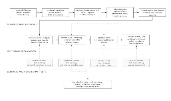
Aligned resamples preserve correlations among observables, scales, matching factors, and fits. Nested resampling separates conditional stochastic errors without pretending shared ensemble variation is independent. The diagram is schematic.

Covariance matrices and conditioning

For data dimension $p$ and only $N_b$ independent blocks, the sample covariance can be noisy or singular. Diagnose its eigenvalue spectrum and effective rank. Remedies include reducing the data vector, increasing independent information, shrinkage toward a declared target, or fitting in a justified principal subspace. A standard well-conditioned shrinkage construction is given by Ledoit and Wolf 2004, pp. 365–411.

Each remedy changes the inferential procedure. Reusing a regularized inverse covariance as if it were known affects goodness-of-fit calibration. Validate parameter coverage with synthetic data that repeats covariance estimation and regularization.

Adversarial failure: intact marginals with destroyed pairing

Let block-level observables satisfy

$$\operatorname{var}(A)=\operatorname{var}(B)=1, \qquad \operatorname{cov}(A,B)=0.99.$$

Aligned resampling gives $\operatorname{var}(A+B)=3.98$ and $\operatorname{var}(A-B)=0.02$. Randomly permuting the block labels of $B$ before resampling leaves both marginal histograms unchanged but drives both variances toward $2$. It therefore understates the standard error of $A+B$ by about $29\%$ and overstates that of $A-B$ by a factor of $10$. A pipeline that checks only marginals will pass this injected defect; a joint-covariance and aligned-resample comparison must reject it.

Observable-level validation checklist

• Preserve a common block or stream identifier across every component derived from shared configurations or calibration data.
• Scan block length using the target nonlinear estimator, not only its fastest input, and retain enough independent units to estimate the requested covariance rank.
• Rerun transformations, fits, scale conversion, and matching inside each jackknife or bootstrap replicate.
• Compare delta-method, block-jackknife, and block-bootstrap covariance on a Gaussian fixture with an analytic answer.
• Inspect covariance eigenvalues, effective rank, and the stability of final observables under declared conditioning choices.
• Inject the block-label permutation above and verify that joint covariance or aligned resampling detects both the sum and difference failures.

Common pitfalls

Resampling timeslices instead of configurations. Timeslices in a correlator are components of one measurement vector, not independent observations.

Choosing a block length from one fast quantity. The derived estimator may overlap a slower mode. Recheck its influence direction and tail.

Adding a shared scale error after joint resampling. If scale variation already entered every resample, adding it again double counts the same source.

Learning outcomes

1. Given an ordered multivariate chain and a nonlinear observable, choose a defensible resampling unit and reproduce its analytic or synthetic covariance with the full transformation rerun in every replicate.
2. Given a noisy or singular covariance and the paired-marginal adversary above, diagnose rank loss, broken pairing, or bias and show quantitatively how the defect changes the final observable uncertainty.

Exercises

1. Let $A=10$, $B=5$, $\operatorname{var}A=1$, $\operatorname{var}B=0.25$, and $\operatorname{cov}(A,B)=0.4$. Estimate $\operatorname{var}(A/B)$.

Solution

$1/25+100(0.25)/625-2(10)(0.4)/125=0.04+0.04-0.064=0.016$.

2. Why must a fit be repeated inside each jackknife sample?

Solution

The fitted parameters are nonlinear functions of all data components and their covariance. Repeating the full fit propagates both changes consistently; deleting only from a post-fit scalar does not.

References

• Efron, B., and Tibshirani, R. J. (1993). An Introduction to the Bootstrap. Chapman & Hall/CRC. DOI.
• Geyer, C. J. (1992). Practical Markov chain Monte Carlo. Statistical Science, 7, 473–483. DOI.
• Ledoit, O., and Wolf, M. (2004). A well-conditioned estimator for large-dimensional covariance matrices. Journal of Multivariate Analysis, 88, 365–411. DOI.