Scale Setting and Dimensionless Ratios

Lattice simulations return dimensionless quantities such as $aM$, $r/a$, or ratios of matrix elements. The conversion depends on the reference quantity’s mass dimension: for an energy or inverse length $X$, $a=(aX)_{\mathrm{lat}}/X_{\mathrm{ref}}$, whereas for a length $\ell$, $a=\ell_{\mathrm{ref}}/(\ell/a)_{\mathrm{lat}}$. The uncertainty in the reference, the interpolation to tuned parameters, and correlations with every target observable must be propagated. A quantity used to tune parameters or set the scale cannot simultaneously be advertised as an independent prediction.

Required background. Euclidean Correlators and Spectral Information supplies dimensionless lattice energies. Bare Parameters, Tuning Conditions, and Continuum Targets distinguishes tuning inputs from held-out predictions.

Helpful background. Scheme Transformations and RG Invariants explains when a reference scale is conventional and how dimensionless predictions remain invariant.

In the chapter’s observable-chain table, this page covers the scale-setting stage and exposes circular inputs before they reach a continuum fit.

Scale setting is a map from ratios to units

First suppose $X$ and $Y$ both have mass dimension one, so a simulation determines $x=aX$ and $y=aY$. If the external or conventional reference value of $X$ is $X_{\mathrm{ref}}$, then

$$a=\frac{x}{X_{\mathrm{ref}}}, \qquad Y_{\mathrm{pred}}=\frac{y}{a} =\frac{y}{x}X_{\mathrm{ref}}.$$

The second form is scientifically clearer: the lattice predicts the dimensionless ratio $Y/X$, while $X_{\mathrm{ref}}$ assigns units. The continuum analysis should therefore be performed on dimensionless ratios whenever possible and unit conversion applied at the end.

More generally, if $X$ has nonzero mass dimension $d$ and the simulation reports $x=a^dX$, then $a=(x/X_{\mathrm{ref}})^{1/d}$. The length formula follows from $d=-1$; for a flow-time reference it gives $a=\sqrt{t_{0,\mathrm{ref}}/(t_0/a^2)_{\mathrm{lat}}}$. Writing the dimension explicitly prevents the common mistake of applying the energy formula to a reported length such as $r/a$ or to a squared length such as $t_0/a^2$.

Scale conventions. Natural units and the site-wide conventions apply. The reference observable, its physical or conventional value, the ensemble interpolation, the mass dependence, the renormalization scheme if relevant, and all shared inputs are local data. This page uses no mutable world average; concrete values are examples only.

For small fluctuations, the variance of $Y=(y/x)X_{\mathrm{ref}}$ is

$$\begin{aligned} \operatorname{Var}(Y) &\simeq \left(\frac{X_{\mathrm{ref}}}{x}\right)^2\operatorname{Var}(y) +\left(\frac{X_{\mathrm{ref}}y}{x^2}\right)^2\operatorname{Var}(x) +\left(\frac yx\right)^2\operatorname{Var}(X_{\mathrm{ref}})\\ &\quad -2\frac{X_{\mathrm{ref}}^2y}{x^3}\operatorname{Cov}(x,y) +2\frac{X_{\mathrm{ref}}y}{x^2}\operatorname{Cov}(y,X_{\mathrm{ref}}) -2\frac{X_{\mathrm{ref}}y^2}{x^3}\operatorname{Cov}(x,X_{\mathrm{ref}}). \end{aligned}$$

Often the external $X_{\mathrm{ref}}$ is independent of the simulation, making the last two covariances zero, but $x$ and $y$ are measured on the same configurations and are not independent. Resampling the entire scale-and-target pipeline preserves this covariance more safely than combining marginal errors afterward.

Reference quantities and what they control

A useful reference has high statistical precision, mild finite-volume and cutoff effects, a clean definition across ensembles, and a reliable connection to the desired physical or conventional units. No reference is universally optimal.

Spectral references. A stable mass or decay quantity is physically transparent but can depend strongly on the simulated masses and may share correlator systematics with the target.

Static-force references. A length such as the Sommer scale $r_0$, defined implicitly by $r_0^2F(r_0)=c$, is precise in gauge calculations but depends on the chosen constant $c$ and the force interpolation Sommer 1994.

Gradient-flow references. Flowed gauge observables define scales such as $t_0$ or $w_0$ through chosen dimensionless conditions. Positive flow time smooths ultraviolet fluctuations, but the condition and flow discretization remain part of the finite-$a$ definition. The construction of $t_0$ is given by Lüscher 2010, §§2–3, while the derivative-based $w_0$ definition and a mass-independent scale analysis are given by Borsányi et al. 2012, §§3–4. A flow scale is not the operator-renormalization scale $\mu$ unless an explicit matching relation is supplied.

Finite-volume references. A box-defined coupling or energy can be used recursively and is natural for step scaling. Its physical-volume condition and boundary scheme must travel with the number.

Comparing two references through a dimensionless continuum combination is a powerful cross-check: examples include $Mr_0$, $r_0/w_0$, or $\sqrt{t_0}/w_0$. Writing $X_1/X_2$ is appropriate only when the two quantities have the same mass dimension. A disagreement at finite $a$ may reflect different cutoff artifacts; a disagreement after controlled extrapolation signals mistuning, underestimated uncertainty, or inconsistent definitions.

Mass-dependent and mass-independent prescriptions

In a mass-dependent prescription, each ensemble or simulated mass point gets its own $a$ from the reference measured there. This can be convenient for interpolation but mixes mass dependence of the reference with cutoff dependence of the lattice spacing.

In a mass-independent prescription, $a$ is assigned at fixed bare gauge coupling after interpolating or extrapolating the reference to a common set of renormalized masses. All ensembles sharing that bare coupling then share the same $a$. This keeps the regulator scale separate from intentional mass variation but introduces correlated interpolation uncertainty.

Neither prescription is intrinsically correct for every problem. The choice must match the constant-physics definition, and conversion between prescriptions should leave continuum dimensionless predictions unchanged within uncertainty. A hidden mixture—for example, mass-dependent $a$ in one observable and mass-independent $a$ in another—creates spurious slopes.

A correlated two-observable example

Suppose an ensemble yields

$$x=aX=0.2500\pm0.0020, \qquad y=aY=0.3750\pm0.0030,$$

with correlation coefficient $\rho_{xy}=0.8$. Then $y/x=1.5$. Ignoring covariance gives relative variance

$$\left(\frac{\sigma_{y/x}}{y/x}\right)^2 =\left(\frac{0.0030}{0.3750}\right)^2 +\left(\frac{0.0020}{0.2500}\right)^2 =1.28\times10^{-4}.$$

Thus an independent-error treatment would give

$$\frac yx=1.5000\pm0.0170.$$

Including covariance subtracts

$$2\rho_{xy} \frac{0.0030}{0.3750} \frac{0.0020}{0.2500} =1.024\times10^{-4},$$

leaving a much smaller variance. This is not a reason to expect cancellation; it is a warning that shared data can materially change the result in either direction. The covariance must be estimated reliably and propagated through all tuning and continuum fits.

Numerically, the correlated result is

$$\frac yx=1.5000\pm0.0076,$$

so dropping the positive correlation more than doubles the standard uncertainty in this fixture.

If $X_{\mathrm{ref}}=400$ MeV is treated as exact in this synthetic example, then

$$a^{-1}=1.600\pm0.013\ \text{GeV}, \qquad Y=600.0\pm3.0\ \text{MeV}.$$

The value $400$ MeV is an illustrative convention, not empirical input. If it carried uncertainty, that additional term and any correlation with the simulated inputs would have to be included.

Circularity and hidden input reuse

Three roles must be recorded separately:

Role	Function	May it validate itself?
Tuning input	Selects bare masses or couplings	No
Scale input	Assigns units to dimensionless results	No
Prediction or validation	Tests the tuned, scaled theory	Yes, if withheld from the first two roles

If $M_A$ participates in the coupled tuning and scale conditions, reproducing it is by construction and is not a held-out prediction. The independent conditions must still be sufficient to determine all parameters being fixed. A ratio $M_B/M_A$ for a state $B$ not used in tuning is an actual prediction. If several physical inputs are needed to define the theory, all are inputs; precision does not turn them into outputs.

Mutable phenomenological averages and the choice among experimental inputs belong to the relevant physics volume or Research. The durable method here is the separation of roles and the covariance-preserving map.

Adversarial failure cases

A different scale per observable. Choosing whichever reference makes each target smooth destroys a common physical unit system. Use one declared prescription and compare alternatives as systematic tests.

Reference interpolation ignored. If $x$ is evaluated at tuned masses obtained from the same data, its uncertainty includes tuning covariance.

Flow time confused with $\mu^{-2}$. A smoothing scale can define a reference length; operator renormalization at scale $\mu$ requires a separate scheme and matching statement.

Ratios formed after independent fits. Fitting $x$ and $y$ separately and combining only marginal errors can lose large covariance. Use joint fits or paired resamples.

Physical units introduced before continuum fitting. This can duplicate scale uncertainty across axes and ordinates. Fit dimensionless quantities with shared scale variables or nuisance parameters.

The complete chain below shows why scale setting is neither the first nor the last inference step. Inspect the direct route and the optional step-scaling detour, then the four failure exits. A reference quantity assigns units, but a second quantity outside the defining inputs must test the tuned and renormalized calculation.

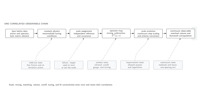
A continuum prediction requires a tuned bare trajectory, a regulator-consistent calculation, and a renormalized observable in a named scheme. When momentum-space lattice perturbation theory is used, its propagators, vertices, and Brillouin zone must be retained unless a controlled matching or subtraction justifies a continuum replacement. Step scaling or scheme conversion is optional when the matching scale is already suitable. The failure exits reject an untuned trajectory, an unjustified continuum propagator inside a lattice loop, a defining input counted as a prediction, and a one-spacing or unsupported extrapolation. Schematic, not to scale.

Observable-level validation checklist

Before quoting a dimensionful prediction, verify:

• the directly measured dimensionless quantities and their joint covariance are available;
• the reference definition, external value, and reason for choosing it are explicit;
• tuning, scale setting, and validation use noncircular roles;
• mass-dependent or mass-independent treatment is consistent across ensembles;
• finite-volume and cutoff effects of the reference are controlled;
• interpolation and external-reference uncertainty are propagated;
• a second reference gives a compatible continuum ratio;
• unit conversion is applied after, or jointly with, the continuum fit without double counting; and
• the unscaled dimensionless result is reported so future reference updates need no reanalysis of raw data.

Exercises

1. Correlated ratio. Derive

$$\frac{\operatorname{Var}(y/x)}{(y/x)^2} \simeq \frac{\sigma_y^2}{y^2} +\frac{\sigma_x^2}{x^2} -2\frac{\operatorname{Cov}(x,y)}{xy}.$$

Solution

Linearize $r=y/x$: $\mathrm dr=(1/x)\mathrm dy-(y/x^2)\mathrm dx$. Contracting this gradient with the $2\times2$ covariance matrix and dividing by $r^2$ gives the stated expression.

2. Identify the prediction. A calculation tunes $M_\pi/M_\Omega$ and $M_K/M_\Omega$, then sets the scale with $M_\Omega$. Which of these three masses is predicted?

Solution

None is an independent prediction: two ratios tune the mass parameters and $M_\Omega$ assigns units. Another observable, such as a decay constant or a different mass ratio not used in tuning, is needed for validation.

What you can now do

You should now be able to convert dimensionless lattice results using an independent reference, preserve shared covariance, and identify circular input reuse. Continue with Nonperturbative Renormalization, Mixing, and Step Scaling to attach a scheme and scale to bare operators before the final continuum analysis.

References

• Borsányi, Szabolcs, Stephan Dürr, Zoltán Fodor, Christian Hoelbling, Sándor D. Katz, Stefan Krieg, Thorsten Kurth, Laurent Lellouch, Thomas Lippert, Craig McNeile, and Kalman K. Szabó. “High-Precision Scale Setting in Lattice QCD.” Journal of High Energy Physics 2012, no. 09 (2012): 010. doi:10.1007/JHEP09(2012)010.
• Lüscher, Martin. “Properties and Uses of the Wilson Flow in Lattice QCD.” Journal of High Energy Physics 2010, no. 08 (2010): 071. doi:10.1007/JHEP08(2010)071.
• Sommer, Rainer. “A New Way to Set the Energy Scale in Lattice Gauge Theories and Its Applications to the Static Force and $\alpha_s$ in SU(2) Yang–Mills Theory.” Nuclear Physics B 411, nos. 2–3 (1994): 839–854. doi:10.1016/0550-3213(94)90473-1.