Light-Front Fock Space, Wavefunctions, and Bound-State Equations

Light-front Fock amplitudes are the coefficients of a regulated Hamiltonian eigenstate expanded at fixed $x^+$. Their longitudinal fractions and relative transverse momenta separate internal motion from the total momentum, so the same coupled equations determine a state in every kinematically related frame. They encode masses and matrix elements through an invariant-mass equation, but they are not equal-time wavefunctions and are not themselves regulator-independent observables. A physical form factor additionally requires a matched current and control of omitted Fock sectors and zero modes.

Required background. Light-Front Coordinates and Quantization supplies the invariant-mass operator and internal momentum variables. Fock Space, Vacuum, and Particle Number supplies occupation-number states, creation operators, and state normalization.

Helpful background. Bethe–Salpeter and Faddeev Bound-State Equations provides a covariant amplitude with a different relative-time structure; the comparison prevents the two objects from being identified without a projection and matching map.

Internal variables and Fock normalization

Convention and regulator card. This page uses $x^\pm=(x^0\pm x^3)/\sqrt2$, one-particle normalization $\langle p',\lambda'|p,\lambda\rangle =2p^+(2\pi)^3\delta(p'^+-p^+)\delta^{(2)}(\mathbf p'_\perp-\mathbf p_\perp) \delta_{\lambda'\lambda}$, and a fixed total $P^+>0$. A calculation must state its longitudinal endpoint and zero-mode prescription, transverse cutoff, Fock-sector set, basis scale, and current renormalization. The formulas below use a scalar basis for clarity; spin, color, and identical- particle factors are restored explicitly in an application.

For an $n$-particle component define

$$p_i^+=x_iP^+, \qquad \mathbf p_{\perp i}=x_i\mathbf P_\perp+\mathbf k_{\perp i},$$

with $x_i>0$, $\sum_i x_i=1$, and $\sum_i\mathbf k_{\perp i}=0$. A convenient internal measure is

$$\mathrm d\Gamma_n =16\pi^3\delta\!\left(1-\sum_i x_i\right) \delta^{(2)}\!\left(\sum_i\mathbf k_{\perp i}\right) \prod_{i=1}^n\frac{\mathrm dx_i\,\mathrm d^2k_{\perp i}}{16\pi^3}.$$

With basis symmetrization factors understood, expand a state of helicity $\lambda$ as

$$|\Psi(P),\lambda\rangle =\sum_n\sum_{\{\lambda_i\}} \int\!\mathrm d\Gamma_n\, \frac{\psi_{n,\lambda}(x_i,\mathbf k_{\perp i},\lambda_i)} {\sqrt{x_1\cdots x_n}} |n;p_i,\lambda_i\rangle .$$

The total-state normalization reduces to

$$1=\sum_n\sum_{\{\lambda_i\}} \int\!\mathrm d\Gamma_n\, \left|\psi_{n,\lambda}(x_i,\mathbf k_{\perp i},\lambda_i)\right|^2.$$

Each term is a Fock-sector probability only within the declared regulator, gauge, basis, and field definition. Changing the cutoff or applying a unitary Hamiltonian transformation redistributes norm among sectors while leaving properly matched observables invariant. The boost-invariant variables, normalization choices, and Fock expansion are derived in Brodsky, Pauli, and Pinsky 1998, §§ 3A–3B and Appendix B, arXiv PDF pp. 35–42 and 172–173.

Support is more than a notation rule. Endpoint behavior as $x_i\to0$ can make the kinetic mass and kernels singular, while the separate $p^+=0$ sector is not obtained simply by evaluating an ordinary wavefunction at $x_i=0$. Any small-$x$ cutoff or endpoint ansatz is therefore part of the regulator.

The invariant-mass equation couples sectors

Insert the expansion into

$$\left(2P^+P^- -\mathbf P_\perp^2\right)|\Psi(P)\rangle =M^2|\Psi(P)\rangle.$$

For free constituents the internal mass is

$$\mathcal M_{0,n}^2 =\sum_{i=1}^n\frac{m_i^2+\mathbf k_{\perp i}^2}{x_i}.$$

Projecting onto each basis sector gives the coupled equations

$$\left[M^2-\mathcal M_{0,n}^2\right]\psi_n(z_n) =\sum_{n'}\int\!\mathrm d\Gamma_{n'}\, K_{nn'}(z_n,z_{n'};\boldsymbol\Lambda)\psi_{n'}(z_{n'}),$$

where $z_n$ denotes all internal labels and $\boldsymbol\Lambda$ denotes every regulator. The kernel contains particle-number-changing vertices, instantaneous terms obtained from constrained fields, counterterms, and any effective interactions induced by omitted sectors. The total momentum drops out only if the regulator and counterterms respect the kinematical boosts. This is an immediate frame-independence check.

A Fock truncation replaces the infinite coupled system by a finite or numerically representable one. It does not merely discard small probabilities: virtual transitions through the omitted sectors renormalize self-energies, vertices, and composite currents. The mass operator and its sector equations are developed in Hiller 2016, §§ 2.3 and 3.1–3.4, preprint pp. 10–29, PDF.

The Fock-space branch of the shared map below records that omitted sectors induce Hamiltonian and current operators. State normalization therefore precedes, but cannot replace, matching and held-out observable tests. The structured regulator table gives the equivalent row-by-row requirements.

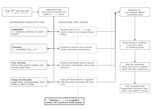
Fock-sector truncation removes virtual intermediate states and thereby induces effective interactions and current corrections. In this schematic, that branch joins the other regulator obligations only at a matched Hamiltonian and must pass spectral, current, Ward, frame, and symmetry tests before joint limits; the map is not to scale.

An exactly solvable two-body model

The following rank-one model separates exact light-front algebra from claims about a particular local QFT. Take two equal-mass scalar constituents and the two-body measure

$$\mathrm d\Gamma_2 =\frac{\mathrm dx\,\mathrm d^2k_\perp}{16\pi^3}, \qquad \mathcal M_0^2(x,\mathbf k_\perp) =\frac{m^2+\mathbf k_\perp^2}{x(1-x)}.$$

Choose a target $M_*^2<4m^2$ and a normalized function

$$\phi_*(x,\mathbf k_\perp) =\mathcal N \,x(1-x) \exp\!\left[-\frac{\mathbf k_\perp^2} {2\beta^2x(1-x)}\right], \qquad \beta>0.$$

Direct Gaussian integration gives

$$1=\int\!\mathrm d\Gamma_2\,|\phi_*|^2 =\frac{\mathcal N^2\beta^2}{2240\pi^2}, \qquad \mathcal N=\frac{8\pi\sqrt{35}}{\beta}.$$

Now set

$$f(z)=\left[\mathcal M_0^2(z)-M_*^2\right]\phi_*(z), \qquad g^{-1}=\int\!\mathrm d\Gamma_2\, f(z)\phi_*(z),$$

and define the attractive separable kernel $K(z,z')=-g f(z)f(z')$. The bound-state equation written as

$$\left[\mathcal M_0^2(z)-M^2\right]\psi(z) =g f(z)\int\!\mathrm d\Gamma_2'\,f(z')\psi(z')$$

has the exact normalized solution $M^2=M_*^2$ and $\psi=\phi_*$. Substitution is the check: the integral equals $g^{-1}$, so both sides are $[\mathcal M_0^2-M_*^2]\phi_*$. The model is intentionally constructed; it tests normalization, kernel signs, and the spectral code, not locality, renormalizability, or phenomenological accuracy.

Currents turn amplitudes into observables

In a Drell–Yan frame with $q^+=0$, the plus component of a correctly matched current often admits a diagonal overlap representation. For a two-body state in which constituent 1 carries unit charge and constituent 2 is a spectator,

$$F(Q^2) =\int\!\mathrm d\Gamma_2\, \psi^*\!\left(x,\mathbf k_\perp+(1-x)\mathbf q_\perp\right) \psi(x,\mathbf k_\perp), \qquad Q^2=\mathbf q_\perp^2.$$

For the exact Gaussian model above,

$$F(Q^2) =140\int_0^1\!\mathrm dx\,x^3(1-x)^3 \exp\!\left[-\frac{Q^2(1-x)}{4\beta^2x}\right].$$

It follows without numerical integration that

$$F(0)=1, \qquad F(Q^2)=1-\frac{Q^2}{3\beta^2}+O(Q^4).$$

The charge normalization independently checks the state normalization and momentum shifts. The overlap representation traces back to the Drell–Yan and West relations Drell and Yan 1970, pp. 181–185, West 1970, pp. 1206–1209.

The word “matched” is essential. In a truncated theory the physical current has the form

$$J_R^\mu =Z_JJ_{\mathrm{basis}}^\mu +\sum_a c_a(\boldsymbol\Lambda)\,\mathcal O_a^\mu,$$

with operators allowed by the residual symmetries. The $q^+=0$ choice can remove ordinary pair-creation terms from a diagonal overlap, but zero modes, instantaneous contributions, and operators induced by omitted sectors may remain. One current component agreeing at one kinematic point is not proof of covariance. Current normalization and the overlap formulas, including their normalization dependence and zero-mode caveat, are given in Hiller 2016, § 2.4, preprint pp. 11–13, PDF.

Distribution amplitudes and parton distributions are likewise projections or bilinears of renormalized amplitudes with a declared scale and operator definition. Their perturbative factorization and evolution belong to Perturbative QFT and Scattering; hadron interpretation belongs to the relevant phenomenology volume. This page develops the Hamiltonian amplitude and current-matching interface.

Adversarial failure: a normalized wavefunction with an unnormalized current

Suppose a truncated state satisfies $\sum_n\int\mathrm d\Gamma_n|\psi_n|^2=1$ to machine precision, but a bare one-body current gives $F(0)=0.93$. Multiplying the final curve by $1/0.93$ repairs one fitted point, not the current. It can hide missing sector operators and need not restore the Ward identity, frame independence, or the other current components.

The repair is to choose renormalization conditions for the current, include all allowed induced operators at the working accuracy, and reserve at least one momentum transfer, current component, or frame as a held-out test. State normalization and charge normalization are related checks, not substitutes.

Observable-level validation

• Support and norm: verify $x_i>0$, both momentum-sum delta functions, and the sector probabilities; report excluded endpoints and zero modes.
• Spectral equation: substitute the numerical eigenvector into every retained sector equation and bound the residual in a declared norm.
• Kinematical boosts: repeat at different external $P^+$ and $\mathbf P_\perp$; the extracted $M^2$ and internal amplitudes must agree.
• Current: enforce the chosen charge or Ward condition, then test a held- out component, frame, or momentum transfer.
• Truncations: vary longitudinal, transverse, basis, and Fock-sector axes separately; renormalize consistently at each point.
• Independent route: compare a mass or form factor with an exact model, perturbation theory in a controlled regime, or a matched Euclidean or equal-time calculation.

You should now be able to (1) normalize a truncated Fock expansion and derive the coupled invariant-mass equation, and (2) distinguish its regulator- dependent amplitudes from a matched physical current matrix element. DLCQ and Basis Light-Front Quantization turns these equations into finite matrices; Light-Front Regulators, Counterterms, and Symmetry Restoration develops their renormalization. Covariant Bethe–Salpeter amplitudes remain with the nonperturbative functional-equation volume.

Exercises

Check the free two-body threshold

Show that $\mathcal M_0^2=(m^2+\mathbf k_\perp^2)/[x(1-x)]\ge4m^2$ and determine when equality holds.

Solution

For $0<x<1$, $x(1-x)\le1/4$, with equality at $x=1/2$. Also $\mathbf k_\perp^2\ge0$. Therefore

$$\mathcal M_0^2 \ge\frac{m^2}{x(1-x)}\ge4m^2.$$

Equality requires both $x=1/2$ and $\mathbf k_\perp=0$. A normalizable state with $M^2<4m^2$ is consequently bound relative to the free two-particle continuum in this model.

Reproduce the Gaussian form-factor slope

Differentiate the one-dimensional expression for $F(Q^2)$ at $Q^2=0$ and verify the coefficient shown above.

Solution

Differentiation under the integral is allowed because the derivative is integrable:

$$F'(0) =-\frac{140}{4\beta^2} \int_0^1\!\mathrm dx\,x^2(1-x)^4 =-\frac{35}{\beta^2}\frac{1}{105} =-\frac{1}{3\beta^2}.$$

The normalization follows separately from $140\int_0^1x^3(1-x)^3\,\mathrm dx=1$. A code that misses the spectator shift $(1-x)\mathbf q_\perp$ fails one or both checks.

References

• Brodsky, Stanley J., Hans-Christian Pauli, and Stephen S. Pinsky. 1998. “Quantum Chromodynamics and Other Field Theories on the Light Cone.” Physics Reports 301: 299–486. DOI. Open PDF.
• Drell, Sidney D., and Tung-Mow Yan. 1970. “Connection of Elastic Electromagnetic Nucleon Form Factors at Large $Q^2$ and Deep Inelastic Structure Functions near Threshold.” Physical Review Letters 24: 181–185. DOI.
• Hiller, John R. 2016. “Nonperturbative Light-Front Hamiltonian Methods.” Progress in Particle and Nuclear Physics 90: 75–124. DOI. Open PDF.
• West, Geoffrey B. 1970. “Phenomenological Model for the Electromagnetic Structure of the Proton.” Physical Review Letters 24: 1206–1209. DOI.