Links, Plaquettes, and Gauge Invariance

A lattice gauge field assigns a parallel transporter to every oriented link. This replaces the continuum connection by finite group elements while preserving local gauge covariance exactly at spacing $a>0$ . Plaquettes are the smallest closed transports and encode curvature; traces of closed paths are gauge invariant because all site transformations cancel locally.

Required background. Review lattice regulators and target continuum theories for the regulator map and parallel transport and holonomy for path composition and closed-loop traces.

Helpful background. Gauge redundancy and the global form of the gauge group explain why local transformation laws alone do not classify all line operators.

Oriented links are exact parallel transporters

Local convention and regulator card. Work on a finite hypercubic lattice of spacing $a$ with compact group $G$ and unitary representation $R$ . The forward variable $U_\mu(x)$ is assigned to $x\to x+a\hat\mu$ but maps the endpoint fiber back to the base fiber; the reverse link is its inverse. Path factors are written in traversal order, so the rightmost matrix acts first, and traces are normalized by $d_R$ .

Let $U_\mu(x)\in G$ be assigned to the oriented link from $x$ to $x+a\hat\mu$ . We use the standard lattice column-vector convention in which $U_\mu(x)\psi(x+a\hat\mu)$ parallel-transports the endpoint field back to the site $x$ . For $\psi(x)\mapsto \Omega_R(x)\psi(x)$ , covariance therefore demands

U_\mu(x)\longmapsto \Omega(x)U_\mu(x)\Omega(x+a\hat\mu)^{-1}.

The opposite orientation is not an independent variable:

U_{-\mu}(x+a\hat\mu)=U_\mu(x)^{-1}.

For a path $C=(\ell_1,\ldots,\ell_n)$ traversed from $x_i=x_0$ to $x_f=x_n$ , where $\ell_k$ joins $x_{k-1}$ to $x_k$ , define

U(C)=U(\ell_1)\cdots U(\ell_n).

The rightmost matrix acts first on a field at $x_f$ , so the intermediate site transformations telescope and

U(C)\mapsto \Omega(x_i)U(C)\Omega(x_f)^{-1}.

Thus $\bar\psi(x_i)U_R(C)\psi(x_f)$ is gauge invariant. An open path alone is covariant, not invariant. A convention that transports from $x_i$ to $x_f$ instead uses the inverse ordered product and reverses both endpoint matrices; mixing the two conventions is the error to avoid.

This endpoint law and the exact cancellation around closed paths are developed in Gattringer and Lang 2010, ch. 3.

The figure fixes the orientation used throughout the chapter. Follow the arrow around the plaquette and observe that each vertex transformation occurs once with each inverse.

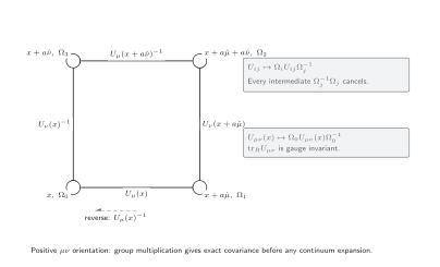
An oriented square plaquette consists of four link matrices; site gauge transformations cancel around the closed product, while reversing any edge replaces its link by the inverse. — With the positive $\mu\nu$ orientation, the plaquette is $U_\mu(x)U_\nu(x+a\hat\mu)U_\mu(x+a\hat\nu)^{-1}U_\nu(x)^{-1}$ . It transforms by conjugation at the base point, so its traced representation character is exactly gauge invariant. The drawing is schematic.

Plaquettes represent regulated curvature

For Hermitian generators $T^a$ with $\operatorname{tr}_R(T^aT^b)=T_R\delta^{ab}$ , choose

U_\mu(x)=\exp\!\left[iag A_\mu^a\!\left(x+\frac{a\hat\mu}{2}\right)T^a\right].

The positively oriented plaquette is

U_{\mu\nu}(x)=U_\mu(x)U_\nu(x+a\hat\mu) U_\mu(x+a\hat\nu)^{-1}U_\nu(x)^{-1}.

Its exact transformation law is

U_{\mu\nu}(x)\mapsto \Omega(x)U_{\mu\nu}(x)\Omega(x)^{-1}.

Consequently $\operatorname{tr}_R U_{\mu\nu}$ and, more generally, the character $\chi_R(U_{\mu\nu})$ are invariant. When the field is smooth on the scale $a$ , the Baker–Campbell–Hausdorff expansion gives

U_{\mu\nu}(x)=\exp\!\left[i a^2g F_{\mu\nu}(x)+O(a^3)\right].

This is an asymptotic relation, not the definition of a plaquette at finite spacing. Exact gauge invariance follows from group multiplication; the interpretation as continuum curvature additionally needs smoothness and a tuned continuum limit.

The group-valued plaquette and closed-loop construction underlying this distinction was introduced by Wilson 1974, pp. 2445–2459.

Closed loops and representation data

For a closed contour $C$ based at $x$ , $U(C)\mapsto\Omega(x)U(C)\Omega(x)^{-1}$ . A normalized Wilson loop in representation $R$ is

W_R(C)=\frac{1}{d_R}\operatorname{tr}_R U_R(C).

Changing the base point cyclically permutes the product and leaves the trace unchanged. Reversing the contour gives

W_R(C^{-1})=W_R(C)^*;

for a real representation it is unchanged. Representation and global form matter: two theories with the same Lie algebra can admit different genuine line operators.

For a periodic lattice, noncontractible loops also record boundary sectors. A gauge transformation periodic only up to a center element can act nontrivially on a winding Polyakov loop even though it leaves every local plaquette invariant. This is why the boundary condition and permitted gauge transformations belong in the convention card.

Worked SU(2) transformation check

Take $G=SU(2)$ with $T^a=\sigma^a/2$ , so $T_F=1/2$ . Under independent matrices $\Omega_0,\Omega_1,\Omega_2,\Omega_3$ at the four corners, write the four positively traversed factors as

\begin{aligned} U_1'&=\Omega_0U_1\Omega_1^{-1}, & U_2'&=\Omega_1U_2\Omega_2^{-1},\\ U_3'&=\Omega_2U_3\Omega_3^{-1}, & U_4'&=\Omega_3U_4\Omega_0^{-1}. \end{aligned}

Their product telescopes:

U_1'U_2'U_3'U_4'=\Omega_0(U_1U_2U_3U_4)\Omega_0^{-1}.

Cyclicity therefore proves $\frac12\operatorname{tr}(U_1U_2U_3U_4)$ invariant. The same calculation catches three frequent implementation errors: using $U$ rather than $U^{-1}$ on a reversed edge, multiplying a path in inconsistent order, or attaching a site transformation to the wrong endpoint.

Gauge convention and observable table

Quantity	Convention	Transformation or check	Status
Forward link	$U_\mu(x):x\to x+a\hat\mu$	$\Omega(x)U_\mu(x)\Omega(x+a\hat\mu)^{-1}$	Gauge covariant
Reverse link	$U_{-\mu}(x+a\hat\mu)=U_\mu(x)^{-1}$	Endpoint law follows by inversion	Gauge covariant
Plaquette	Positive $\mu\nu$ boundary based at $x$	Conjugation by $\Omega(x)$	Gauge covariant
Plaquette trace	$d_R^{-1}\operatorname{tr}_R U_{\mu\nu}$	Unchanged under conjugation	Gauge invariant
Open transporter	$C:x_i\to x_f$ ; $U(C)$ maps the endpoint fiber back to the base point	$\Omega(x_i)U(C)\Omega(x_f)^{-1}$	Not gauge invariant alone
Closed Wilson loop	$d_R^{-1}\operatorname{tr}_R U(C)$	Reverse path gives complex conjugate	Gauge invariant

Adversarial failure: an ordering error hidden by Abelian tests

Consider two consecutive links $U_1:x_0\to x_1$ and $U_2:x_1\to x_2$ . The correct transporter is $U_1U_2$ . A program that instead forms $\widetilde U=U_2U_1$ can pass every test on a $U(1)$ configuration because all matrices and site phases commute; it also passes a non-Abelian test restricted to a constant gauge transformation. Under independent non-Abelian site transformations, however,

\widetilde U'= \Omega_1U_2\Omega_2^{-1}\Omega_0U_1\Omega_1^{-1},

which cannot be reduced to $\Omega_0\widetilde U\Omega_2^{-1}$ . A random-site $SU(2)$ covariance test therefore detects a convention error that an Abelian plaquette test can conceal.

Observable-level validation checklist

Draw the base and endpoint of every factor and verify that $U(C)$ maps the endpoint fiber to the base fiber.
Apply independent random site transformations and require the open-path covariance defect and traced-plaquette invariance defect to vanish to numerical precision.
Reverse a contour and check $W_R(C^{-1})=W_R(C)^*$ in the chosen representation.
On a smooth background, verify $\lVert U_p-I\rVert=O(a^2)$ and $1-\operatorname{Re}\operatorname{tr}U_p/d_R=O(a^4)$ without using this expansion to prove exact invariance.
On a periodic lattice, test contractible and winding loops separately under the allowed center-twisted transformations.

Common pitfalls

Expanding links before proving covariance. The continuum expansion is unnecessary for the exact cancellation and can conceal orientation mistakes. Verify the finite-group transformation first, then expand.

Calling every traced path a local observable. A winding loop can be gauge invariant while remaining sensitive to global boundary sectors and center transformations. Record the contour’s homotopy and boundary condition.

Suppressing representation normalization. $\operatorname{tr}T^aT^b$ , $d_R$ , and the coupling convention jointly determine continuum coefficients. A numerical plaquette without them cannot be translated reliably.

Learning outcomes

Given an oriented path and independent site transformations, construct its ordered transporter, derive its endpoint covariance, and supply the matter fields or trace needed for gauge invariance.
Given $G$ , $R$ , generator normalization, and a plaquette orientation, translate a Wilson-loop convention and verify both contour reversal and the leading smooth-field scaling.

Exercises

Show that the gauge-invariant nearest-neighbor scalar hopping term is $\phi(x)^\dagger U_R(x,\mu)\phi(x+a\hat\mu)+\text{c.c.}$ .

Solution

Transforming the first term gives $\phi^\dagger\Omega_R^\dagger\Omega_RU_R\Omega_R^{-1}\Omega_R\phi$ , so all site matrices cancel. Its complex conjugate is invariant separately.

Prove $\operatorname{tr}_R U(C^{-1})=[\operatorname{tr}_R U(C)]^*$ for a unitary representation.

References

Section titled “References”- Gattringer, C., and Lang, C. B. (2010). Quantum Chromodynamics on the Lattice: An Introductory Presentation, ch. 3. Springer. DOI.
- Wilson, K. G. (1974). Confinement of quarks. Physical Review D, 10, 2445–2459. DOI.
Further reading
Section titled “Further reading”- Kogut, J. B. (1979). An introduction to lattice gauge theory and spin systems. Reviews of Modern Physics, 51, 659–713. DOI.
Original QFT.org content:CC BY 4.0, unless an item supplies different terms. Third-party material retains its own terms.