

Finite Volume as a Controlled Deformation
Finite spatial volume is a controlled infrared deformation only when the box, boundary conditions, interaction range, mass gap, temporal extent, symmetry sector, and order of limits are all part of the definition of the calculation. For a massive local theory with range and , isolated stable-particle effects are usually exponentially small, while on-shell multi-particle propagation produces the power-law dependence that quantization conditions use. Massless fields, long-range forces, zero modes, thresholds, and wrongly ordered limits require different branches; “large volume” by itself is not a hypothesis.
Required background. Euclidean Correlators and Spectral Information supplies the spectral quantities whose volume dependence is measured. Lattice Geometry, Boundaries, and Anisotropy supplies finite-lattice geometry and boundary data.
Helpful background. Boundaries and State Preparation explains how boundary conditions select states rather than merely changing notation.
Scales and states in a spatial box
Section titled “Scales and states in a spatial box”Take a Euclidean lattice with spacing , spatial extents , and temporal extent . Periodic or twisted spatial boundary conditions give
Finite-volume deformation convention. Every limit below holds at fixed renormalized physics with the spatial geometry, boundary phases, temporal extent, interaction range, mass gap, state sector, and limit order stated.
The choices that affect every later formula are:
| Field | Choice used on this page |
|---|---|
| Setting | Zero-temperature Euclidean correlators on a rectangular spatial torus; is finite during data generation but is not identified with inverse temperature |
| Geometry | means the shortest spatial extent when a single size is quoted; periodic boundaries are the default, and twists are displayed explicitly |
| Finite-volume states | within a fixed total-momentum and lattice-irrep sector |
| Range data | is an interaction range, is the longest bulk correlation length allowed by the quantum numbers, and neither is silently identified with the target particle’s Compton wavelength |
| Limit order | First control -wrap effects and take the continuum limit along a line of constant physics; then take at fixed renormalized masses and couplings unless the observable specifies another order |
| Invariant check | An infinite-volume pole, phase shift, or matrix element must be reproduced from at least two volumes or frames by the same branch and normalization |
A useful dimensionless hierarchy is
supplemented by the channel-specific ratios , binding momentum , threshold separations divided by the level uncertainty, and the aspect ratios . The first inequality controls cutoff effects, the next two control spatial images, and the last separates propagation around time from propagation around space. One large product cannot compensate for another small one.
The distinction between exponential and power-law effects is analytic. A loop momentum sum may be written by Poisson summation as
If the contour can be displaced to the nearest massive singularity, each image is exponentially suppressed. If intermediate particles can go on shell, the contour is pinched and the sum–integral difference is only power suppressed. This is the structural separation behind the stable-particle and scattering results proved by Lüscher 1986, Part I, pp. 177–206 and Lüscher 1986, Part II, pp. 153–188.
A free-field benchmark and an interacting warning
Section titled “A free-field benchmark and an interacting warning”For a free scalar of mass in a periodic cubic box,
The zero-momentum one-particle energy is exactly : momentum discretization alone does not shift a free pole mass. A two-particle level is exactly subject to total-momentum conservation. This benchmark detects two common errors immediately: treating all discrete levels as interaction shifts, and inferring a scattering amplitude from free kinematics without a quantization condition.
Interactions change the conclusion in two distinct ways. Virtual massive particles wrapping around the box shift an isolated stable level by terms such as . On-shell two-particle propagation instead shifts nearby levels by powers of whose coefficients contain the scattering amplitude. A shallow bound state introduces the binding length ; its volume dependence is uncontrolled when is not large even if is. Thus the lightest bulk mass, interaction range, and target state size must be recorded separately.
The diagram shows where each hypothesis enters. Inspect the dashed exits: a long-range theory does not pass through the short-range quantization box, and a failed covariance or continuation check stops the claim at the finite-volume data.
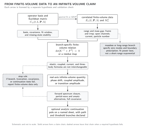
Finite-volume information reaches an infinite-volume claim only through a branch-specific map. Solid arrows show the controlled chain; dashed arrows show the long-range alternative and the stop rule. The image is a schematic, not to scale, and the displayed determinant is structural: its channel, irrep, partial-wave, normalization, and sign conventions must be fixed locally.
Hypothesis, branch, and uncertainty table
Section titled “Hypothesis, branch, and uncertainty table”This table is the structured equivalent of the diagram and the starting record for any finite-volume analysis. A row is usable only when every hypothesis in its second column has been checked.
| Regime | Required hypotheses and branch data | Finite-to-infinite-volume map | Observable-level validation | Dominant uncertainty or failure signal |
|---|---|---|---|---|
| Isolated stable particle or compact bound state | Massive local theory; state stable in the studied sector; ; relevant or ; boundary phases stated | Image or wrapping expansion for the pole energy or matrix element; no scattering inversion | Fit several including subleading images; verify the same infinite-volume pole and temporal-wrap stability | Threshold pinching, a shallow binding scale, or an omitted lighter exchange changes the exponent and coefficient |
| Massless field or long-range force | Zero-mode prescription, Gauss constraint, locality and symmetry properties, box shape, and target infrared observable stated | Prescription-specific sum–integral difference and power expansion | Reproduce an exact point-particle or Ward-identity benchmark and match prescriptions only at common infrared conditions | , shape, or dependence; an exponential fit is an adversarial failure |
| Elastic two-body level | Two stable particles; one open channel; short range; energy below the first omitted inelastic threshold; frame , irrep , partial waves, branch integer, and exponential remainder stated | Elastic quantization condition gives a real-axis phase shift or matrix | Invert correlated levels, then predict held-out levels in another , , or | Inelasticity, long-range exchange, partial-wave truncation, wrong root, or underestimated covariance |
| Moving-frame or spinning two-body level | Little group, subduction convention, spin/helicity basis, multiplicities, parity restrictions, and partial-wave cutoff stated | Irrep-block determinant in the declared basis | Operator overlaps and noninteracting levels match irrep content; enlarge the partial-wave basis | Assigning continuum to one cubic level or dropping an allowed mixed wave |
| Coupled two-body channels | All open and nearby channels, thresholds, state normalization, sheet-sign vector, and unitary parametrization stated | Coupled determinant constrains a matrix amplitude | Elastic decoupling limit, synthetic closure, alternative unitary forms, and multi-frame sensitivity | Sparse levels identify only parameter combinations; a pole becomes ansatz or sheet dominated |
| Current insertion, one to two particles | Renormalized current, finite- and infinite-volume state norms, injected momentum, residue derivative, final-state branch, and shared covariance stated | Lellouch–Lüscher or matrix-residue factor converts to a transition amplitude | Free or solvable density-of-states limit and joint spectrum–current resampling | Missing , derivative, current-renormalization, or spectrum–matrix-element covariance factor |
| Three-particle level or decay bridge | One named formalism; spectator and subchannel basis; symmetrization; two-body pole treatment; regulator and scheme; allowed couplings stated | Three-body determinant gives scheme-dependent intermediate quantities, followed by integral equations for a physical amplitude | Free spectrum, weak-coupling or threshold expansion, scheme cancellation, and independent synthetic closure | Treating as an observable, importing a two-body formula, or inheriting two-body validation |
The table deliberately distinguishes durable formulas from mutable comparisons. Current implementation status for coupled-channel, current, and three-body branches belongs to the Lattice and Hamiltonian Field Theory Research area.
Order of limits is part of the observable
Section titled “Order of limits is part of the observable”For a massive zero-temperature observable, a safe default is
where each limit means a controlled extrapolation, not one simulation point. Other orders can define other physics. Taking before activates zero modes; taking comparable to can mix temporal wrapping with spatial effects; holding fixed while sends the physical volume to zero. Spontaneous symmetry breaking also requires an infinite-volume limit before removing a symmetry-breaking source. These are inequivalent limits, not alternative fit conventions.
Adversarial case. Suppose three volumes with are well fit by . If the target is a shallow bound state with , then throughout. The fit quality cannot license the asymptotic form: the state overlaps strongly with its images, and omitted terms are not ordered. The correct outcome is “finite-volume energies measured; infinite-volume bound state not controlled.”
Observable-level validation
Section titled “Observable-level validation”Before interpreting a finite-volume result, verify all of the following:
- the reported , , , boundary phases, masses, range proxy, frame, irrep, channel set, and order of limits reproduce the analysis input;
- temporal images, spatial images, discretization effects, and excited-state contamination have distinct variations;
- the branch formula is applied only inside its range, threshold, particle-number, and current-insertion hypotheses;
- a correlated forward calculation reproduces all fitted levels and at least one held-out volume, frame, or irrep;
- partial-wave, amplitude-ansatz, zero-mode-prescription, and analytic-branch alternatives are propagated when they can change the observable; and
- the final claim names what remains finite-volume data, what is an infinite-volume real-axis quantity, and what additionally depends on analytic continuation.
What you can now do
Section titled “What you can now do”You can now (1) construct and numerically evaluate the hierarchy , , , , , and threshold separations for a proposed calculation, and (2) assign each observed volume dependence to the exponential, power-law, zero-mode, or uncontrolled row of the table with an explicit stop rule.
Continue to Exponential Finite-Volume Effects for massive wrapping corrections, Massless Fields, Long-Range Forces, and Finite-Volume QED for the power-law exception, or Spectra from Euclidean Correlation Matrices to begin the spectrum-to-amplitude chain. Thermal compactification is a distinct physical problem treated in Thermal and Nonequilibrium QFT.
Exercises
Section titled “Exercises”1. Separate the scales. A calculation has , , , a lightest exchange mass , and a bound-state binding momentum . Using , decide which exponential expansion is less controlled.
Solution
, , and . Bulk temporal wrapping is better suppressed than bulk spatial wrapping, but the bound-state image expansion is the least controlled because . Quoting only would miss the largest state-size effect.
2. Diagnose a limit. Let and take at fixed . Does this produce the infinite-volume continuum theory?
Solution
No. It produces a continuum discretization limit with , not . A line of constant physics requires increasing so that the chosen physical volume remains fixed during the continuum extrapolation, then varying that physical volume for the infinite-volume limit.
References
Section titled “References”- Lüscher, Martin. “Volume Dependence of the Energy Spectrum in Massive Quantum Field Theories. I. Stable Particle States.” Communications in Mathematical Physics 104 (1986): 177–206. DOI.
- Lüscher, Martin. “Volume Dependence of the Energy Spectrum in Massive Quantum Field Theories. II. Scattering States.” Communications in Mathematical Physics 105 (1986): 153–188. DOI.
Original QFT.org content:CC BY 4.0, unless an item supplies different terms. Third-party material retains its own terms.