Resource and Continuum Certification

A scientific resource estimate begins with a renormalized observable and target uncertainty, then chooses spatial spacing, physical volume, local Hilbert dimension, preparation success, evolution time, algorithmic tolerance, measurement repetitions, and logical resources together. Symbolic scaling is conditional on those choices. Logical gates are not physical hardware resources, and neither number establishes continuum accuracy or advantage.

Required background. Verification, error mitigation, and observable certification supplies the accepted error model. Lines of constant physics and continuum extrapolation supplies regulator removal. Convergence, extrapolation, and error certification supplies local-Hilbert convergence.

Helpful background. Encoding fields and truncating local Hilbert spaces supplies qubit, qudit, and operator-support costs.

From physical accuracy to regulator size

Convention and regulator card. Let $O_{\rm cont}$ be a dimensionless renormalized observable, or divide a dimensionful observable by a declared reference scale. The total tolerance $\epsilon_{\rm tot}$ and confidence $1-\alpha_{\rm stat}$ are fixed before resource optimization. Spatial dimension is $d_s$, $N_s=(L/a)^{d_s}$ is the site count, and every asymptotic expression states which physical parameters are held fixed.

Use an additive observable-level allocation,

$$\epsilon_{\rm tot}\ge \epsilon_a+\epsilon_L+\epsilon_{\rm loc} +\epsilon_{\rm prep}+\epsilon_{\rm evol} +\epsilon_{\rm synth}+\epsilon_{\rm noise} +\epsilon_{\rm mit}+\epsilon_{\rm stat}.$$

The triangle inequality makes this conservative and transparent. If correlations or cancellations are used, include their covariance and demonstrate stability rather than silently subtracting errors.

Suppose a controlled regime has leading forms

$$\epsilon_a\le c_a(a\Lambda)^p,\qquad \epsilon_L\le c_Le^{-m_{\rm gap}L},\qquad \epsilon_{\rm loc}\le c_de^{-\kappa d_{\rm loc}}.$$

The last exponential is an illustrative state-dependent local-truncation model, not a universal law. Allocated tolerances imply

$$a\le\Lambda^{-1}\left(\frac{\epsilon_a}{c_a}\right)^{1/p}, \quad L\ge m_{\rm gap}^{-1}\log\frac{c_L}{\epsilon_L}, \quad d_{\rm loc}\ge\kappa^{-1}\log\frac{c_d}{\epsilon_{\rm loc}}.$$

Coefficients and exponents must come from analytic control or a resolved convergence campaign. Near criticality $m_{\rm gap}\to0$, the finite-volume requirement changes qualitatively. A resource estimate that inserts continuum power counting while holding $N_s$ fixed is inconsistent.

Logical resources and success overhead

For a local binary encoding,

$$Q_L=N_s\lceil\log_2d_{\rm loc}\rceil+Q_{\rm anc}+Q_{\rm work}.$$

Logical operation counts should be decomposed,

$$G_L=G_{\rm encode}+G_{\rm prep}+G_{\rm evol} +G_{\rm measure}+G_{\rm uncompute},$$

with $G_{\rm evol}$ derived from the selected algorithm’s norm, commutator, or block-encoding parameters. The field-theory scattering construction of Jordan, Lee, and Preskill 2012 demonstrates why lattice spacing, volume, field digitization, preparation, and scattering precision all enter an asymptotic cost; one should not reuse its scaling outside its theory and accuracy hypotheses.

If an accepted estimate needs $N_{\rm acc}$ successful samples, then

$$N_{\rm raw}= \frac{\Gamma_{\rm mit}N_{\rm acc}} {p_{\rm prep}\,p_{\rm sector}\,p_{\rm alg}},$$

where $p_{\rm prep}$ is state-preparation success, $p_{\rm sector}$ postselection acceptance, $p_{\rm alg}$ any heralded algorithmic success, and $\Gamma_{\rm mit}\ge1$ the mitigation sampling overhead. Correlations and restart costs can increase this further. Classical preprocessing, coefficient generation, compilation, decoding, covariance analysis, and continuum fitting are part of the end-to-end resources.

These are logical, platform-independent quantities. Mapping them to physical qubits, code cycles, wall time, energy, or monetary cost requires a specified error-correction architecture, gate set, physical error model, decoder, and hardware assumptions. Those changing inputs and resulting feasibility statements belong in dated Research evidence.

Resource and evidence boundaries

The figure shows that symbolic complexity and continuum accuracy are different axes. Inspect the gates separating a finite-regulator logical estimate from a continuum-certified result and from a dated matched-baseline comparison.

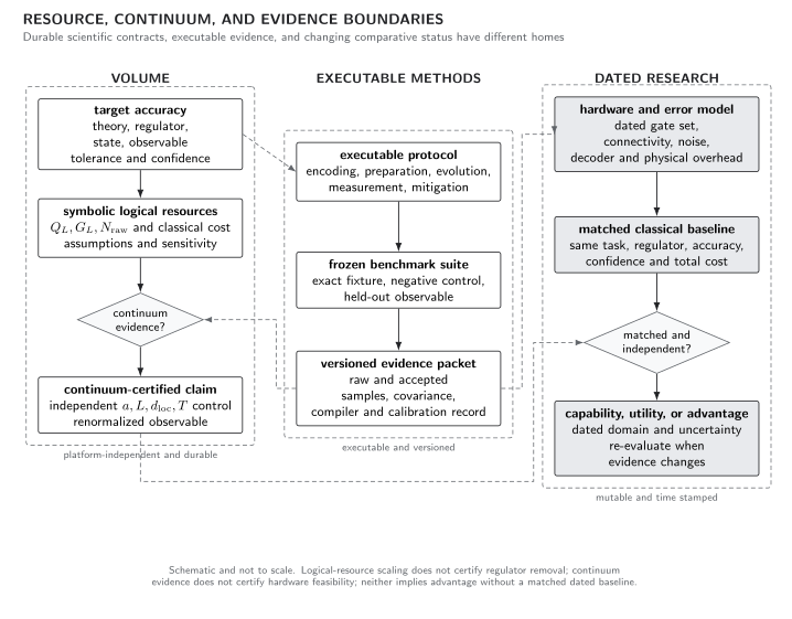
Resource certification owned by this Volume connects observable tolerance to regulator sizes, logical qubits, operations, repetitions, success probabilities, and classical costs. Continuum evidence is a separate gate. Executable estimators require reproducible records, while device-specific physical overhead and matched advantage assessments require dated Research inputs. The map is schematic and contains no hardware forecast.

The canonical claim–resource–evidence record keeps symbolic resources, target error, matched baseline, and evidence ceiling attached to one scientific task.

Sensitivity analysis

A point estimate hides which assumption controls the conclusion. For total resource $R(\vartheta)$ and uncertain input $\vartheta_i$, report a local elasticity

$$S_i=\frac{\partial\log R}{\partial\log\vartheta_i}$$

or a finite-range envelope when derivatives are misleading. Vary the continuum exponent $p$, gap $m_{\rm gap}$, truncation rate $\kappa$, preparation success, Hamiltonian norm, algorithm order, mitigation overhead, and target confidence. Correlated inputs should be varied jointly.

If $R\propto N_s^\gamma$ and the lattice error fixes $a\propto\epsilon_a^{1/p}$ at fixed $L$, then

$$R\propto\epsilon_a^{-\gamma d_s/p}.$$

A modest change in $p$ or spatial dimension can dominate a claimed precision scaling. Report the range supported by data, not only a preferred exponent.

Analytic benchmark: a transparent scalar estimate

Take $d_s=1$, measure all quantities in units of a gap $m=1$, and use the illustrative bounds

$$\epsilon_a=a^2,\qquad \epsilon_L=e^{-L},\qquad \epsilon_{\rm loc}=e^{-d_{\rm loc}}.$$

Allocate $0.005$ to each of these three errors. Then

$$a\le\sqrt{0.005}=0.0707,\quad L\ge\log 200=5.30,\quad d_{\rm loc}\ge\log 200=5.30.$$

Choosing $a=0.070$, $L=5.32$, and integer $d_{\rm loc}=6$ gives $N_s=76$ sites and at least

$$Q_{\rm field}=76\lceil\log_2 6\rceil=228$$

logical field qubits before ancillas. This is not a forecast: the assumed coefficients are synthetic and the gate count, preparation, samples, and error correction are absent. Its purpose is to verify the inference chain and dimensions. A real estimate must fit the coefficients from regulator data, round choices conservatively, and propagate their covariance.

Adversarial failures

Asymptotic gates without target accuracy. A polynomial gate count omits how $a$, $L$, and $d_{\rm loc}$ depend on $\epsilon_{\rm tot}$. It is an algorithmic statement, not a continuum-QFT resource estimate.

Logical-to-physical shortcut. Multiplying logical qubits by a fixed overhead ignores code distance, logical error target, decoder, connectivity, and circuit duration. Keep the logical result durable and route a dated physical mapping to Research.

Preparation omitted from repetitions. A costly adiabatic or postselected state is treated as free for every shot. Include retries, state reuse assumptions, and destructive measurement.

One favorable exponent. A continuum fit cannot distinguish $p=1$ from $p=2$, but only $p=2$ is quoted. Carry both models or acquire enough regulator points to discriminate them.

Observable-level validation checklist

• Fix the renormalized observable, total tolerance, confidence, physical parameters, and limit order.
• Derive $a$, $L$, $d_{\rm loc}$, time window, and preparation quality from separately validated error models.
• Count logical qubits, ancillas, oracle construction, compiled operations, measurements, success amplification, mitigation, and classical processing.
• Include raw repetitions after preparation, postselection, algorithmic success, correlations, and confidence.
• Perform sensitivity or scenario analysis for every uncertain exponent, coefficient, gap, norm, and success probability.
• Keep logical resources separate from device-specific physical overhead and compare quantum and classical workflows only at identical tasks and accuracy.

Exercises

1. Precision scaling

At fixed physical $L$, suppose $\epsilon_a=c(a\Lambda)^2$ and a logical cost scales as $R\propto N_s^3$ in two spatial dimensions. How does $R$ scale with the allocated lattice tolerance?

Solution

$a\propto\epsilon_a^{1/2}$, $N_s=(L/a)^2\propto\epsilon_a^{-1}$, and therefore $R\propto\epsilon_a^{-3}$. Constants depend on $c$, $\Lambda$, and $L$.

2. Success overhead

A protocol needs $10^4$ accepted samples, with $p_{\rm prep}=0.8$, $p_{\rm sector}=0.5$, $p_{\rm alg}=1$, and $\Gamma_{\rm mit}=3$. Find the expected raw runs.

Solution

$$N_{\rm raw}=\frac{3\times10^4}{0.8\times0.5}=75{,}000.$$

This expectation does not include temporal correlations, calibration shots, or failed jobs.

Learning outcomes

After working this page, you should be able to:

• Convert a continuum observable tolerance into spatial size, local dimension, time, logical qubits, operations, repetitions, success overhead, and classical processing under explicit regulator and algorithm hypotheses.
• Compute sensitivity to continuum exponents, gaps, truncation rates, preparation success, mitigation overhead, and algorithm norms, and identify which assumption dominates the resource conclusion.

Handoff

A benchmark ladder for quantum field simulators decides which scientific claim the resulting evidence supports. Error-correction architecture, physical overhead, hardware capability, and advantage comparisons belong in dated Research records.

References

• Jordan, Stephen P., Keith S. M. Lee, and John Preskill. “Quantum Algorithms for Quantum Field Theories.” Science 336 (2012): 1130–1133. doi:10.1126/science.1217069.