Variational Principles and Field-Theory Ansätze

A field-theory ansatz is a controlled variational approximation when its regulated Hilbert space, normalization, exact symmetries, parameter manifold, optimization procedure, residuals, and systematic enlargements are all declared. Rayleigh–Ritz gives an upper bound for energies under precise hypotheses; it does not bound general observables, remove ultraviolet or volume regulators, or prove that a nonlinear optimizer found the best state in the chosen manifold.

Required background. Hilbert-Space Truncation as a Regulator supplies the regulated domain and omitted states. Field Variations and Boundary Terms supplies functional variation, admissible variations, and boundary conditions.

Helpful background. Vacua, States, and Representations supplies the distinction between a state ansatz, a representation, and a physical vacuum claim.

Rayleigh–Ritz controls energies inside a declared space

Variational manifold contract. Specify the prior field regulator and volume; normalized state map $\theta\mapsto|\psi(\theta)\rangle$; exact sectors and constraints; real or complex parameter domain; objective and optimizer; initialization and stopping rules; residual and variance; ansatz enlargement; and the limit in which the target QFT is recovered. Label an energy as a rigorous bound only when the Hamiltonian, domain, and orthogonality hypotheses have been checked.

For a nonzero trial state in the form domain of a self-adjoint Hamiltonian bounded below, the Rayleigh quotient is

$$\mathcal E[\psi] =\frac{\langle\psi|H|\psi\rangle}{\langle\psi|\psi\rangle}.$$

Writing $|\psi\rangle\mapsto|\psi\rangle+|\delta\psi\rangle$ gives

$$\delta\mathcal E =\frac{2\operatorname{Re} \langle\delta\psi|(H-\mathcal E)|\psi\rangle} {\langle\psi|\psi\rangle}.$$

Thus stationarity on a smooth parameter manifold requires the Hamiltonian residual to be orthogonal to every tangent direction:

$$\operatorname{Re}\langle\partial_a\psi| (H-\mathcal E)|\psi\rangle=0.$$

Minimizing over any admissible subset gives $\mathcal E\ge E_0$. Enlarging a nested linear trial space cannot raise its minimum. A sequence of nonlinear manifolds has the same monotonic property only if the manifolds are actually nested and the global minimum is found.

Excited-state bounds require orthogonality to the exact lower eigenspaces or the full min–max construction. Orthogonality only to approximate lower states can produce biased excited energies. The mathematical basis of these ordered Ritz bounds is the min–max principle Reed and Simon 1978, Chapter XIII, §1.

A Gaussian scalar mode is exactly checkable

Consider one regulated scalar mode with $m>0$,

$$H=\frac{p^2}{2}+\frac{m^2q^2}{2}+\frac{\lambda q^4}{4!}, \qquad \lambda\ge0,$$

and the normalized Gaussian

$$\psi_\Omega(q)=\left(\frac{\Omega}{\pi}\right)^{1/4} e^{-\Omega q^2/2}, \qquad \Omega>0.$$

Using $\langle p^2\rangle=\Omega/2$, $\langle q^2\rangle=1/(2\Omega)$, and $\langle q^4\rangle=3/(4\Omega^2)$ gives

$$E_G(\Omega) =\frac{\Omega}{4}+\frac{m^2}{4\Omega} +\frac{\lambda}{32\Omega^2}.$$

Stationarity yields

$$\frac{dE_G}{d\Omega}=0 \quad\Longleftrightarrow\quad \Omega^3-m^2\Omega-\frac{\lambda}{4}=0.$$

At $\lambda=0$, the positive solution $\Omega=m$ gives $E_G=m/2$, the exact oscillator ground energy. At nonzero coupling, solving the cubic and comparing with a basis-diagonalization reference tests normalization, moments, gradients, and optimizer output. The result remains an upper bound for this regulated oscillator; calling it the vacuum energy of a continuum field theory would require restoring all modes and removing every regulator.

For a scalar field, a translationally invariant Gaussian ansatz assigns a kernel or mode frequency $\Omega_k$. Non-Gaussian improvements may add correlated-pair, polynomial, circuit, coupled-cluster, or neural components. Each extension changes both expressivity and optimization geometry. Parameter count alone is not an ordering: the relevant test is whether the old manifold is embedded in the new one and whether both optimizations reach comparable stationarity.

Residual and variance diagnose different failures

For a normalized trial state with energy $E=\langle H\rangle$, define

$$|r\rangle=(H-E)|\psi\rangle, \qquad \sigma_H^2=\langle r|r\rangle =\langle H^2\rangle-E^2.$$

Expanding in exact energy eigenstates shows that at least one spectral value lies within $\sigma_H$ of $E$. This statement does not identify which eigenvalue when the spectrum is crowded. If an independently established lower bound $E_1^{\mathrm{lb}}>E$ on the first excited energy is available, Temple’s inequality sharpens the ground-state statement:

$$E-\frac{\sigma_H^2}{E_1^{\mathrm{lb}}-E} \le E_0\le E.$$

The denominator condition is essential; inserting an approximate gap without a valid lower bound destroys the rigorous claim.

A small parameter gradient is weaker than a small Hilbert-space residual. It means only that $r$ is orthogonal to the ansatz tangent space. The residual can point almost entirely in omitted variational directions. Measuring or estimating $\sigma_H$ and enlarging the manifold probe this failure.

Symmetry and normalization belong inside the ansatz

There are three clean strategies for an exact symmetry: construct invariant states, project an ansatz with a group projector, or optimize in a fixed irrep. A penalty such as $\kappa\langle G^2\rangle$ changes the Hamiltonian at finite $\kappa$ and must be extrapolated or bounded. A small $\langle G\rangle$ alone does not imply a small constraint norm; monitor $\langle G^2\rangle=\|G\psi\|^2$ or the exact projector residual.

Normalization can be analytic, enforced by coordinates, or included through a generalized metric. Near-null tangent directions make the optimization ill-conditioned. Record the tangent Gram matrix

$$S_{ab}=\langle\partial_a\psi\mid\partial_b\psi\rangle -\langle\partial_a\psi\mid\psi\rangle \langle\psi\mid\partial_b\psi\rangle$$

and the regularization used to solve natural-gradient or time-dependent equations. Discarding small singular values changes the variational manifold and must be tested as another cutoff.

Time-dependent variation is projected dynamics

The Dirac–Frenkel condition projects the Schrödinger residual onto the tangent space:

$$\langle\partial_a\psi| \left(i\frac{d}{dt}-H\right)|\psi\rangle=0.$$

McLachlan’s formulation minimizes the norm of the same residual over allowed velocities. They agree under common regularity and complex-tangent conditions but can differ on restricted real manifolds. The original least-error principle is stated by McLachlan 1964, pp. 39–44; modern geometric treatments emphasize that the projected flow inherits the manifold’s tangent metric and singularities Lubich 2008, Chapters II–III.

Energy conservation inside projected real-time evolution, when present, does not prove trajectory accuracy. Track the instantaneous Schrödinger residual, conserved charges, norm, and a held-out correlator against ansatz enlargement.

The convergence map distinguishes a bound from a prediction

The variational branch in the shared map certifies only those ordered energies covered by the min–max hypotheses. It must rejoin effective observables and held-out tests before supporting claims about other quantities.

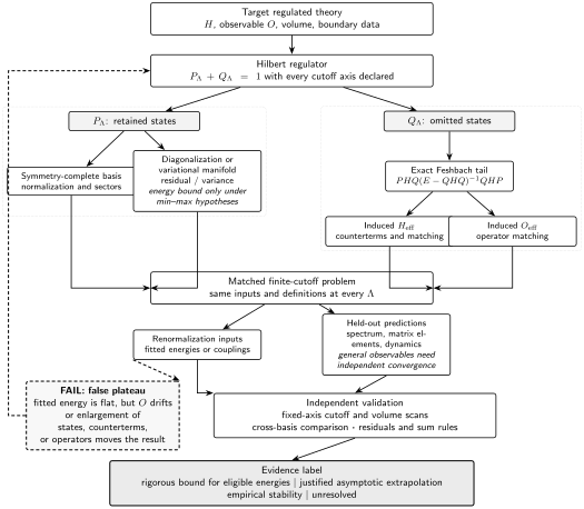
Variational minimization can supply monotone upper bounds for eligible energies, while residuals and ansatz enlargement diagnose the chosen manifold. General matrix elements and dynamics still require effective operators, independent cutoffs, and held-out checks; the schematic false plateau is not to scale.

Minimum truncation certification record

Required fields for a truncation result and the test that can falsify each field.

Field	Required declaration	Independent test	Failure signal
Target	Hamiltonian, prior regulator, volume, boundary data, observable	Units and free or exact limit	Changing target across cutoff points
Projectors	PΛ, QΛ, all cutoff axes, limit order	State counts and nestedness	Unidentified omitted states
Basis and sectors	Normalization, Gram matrix, null removal, exact charges	Hermiticity and selection rules	Duplicates or broken constraints
Induced Hamiltonian	Derived operator basis and approximation order	Omitted-state toy model or perturbative coefficient	Drift incompatible with the declared tail
Counterterms	Inputs, running coefficients, and no-double-counting rule	Refit protocol at every cutoff	A fitted datum presented as a prediction
Variational status	Manifold, optimizer, symmetry, bound hypotheses	Residual, variance, and ansatz enlargement	Energy plateau with a large residual
Effective observables	Projected and induced operator terms	Sum rule or matched matrix element	Spectrum stable while the observable drifts
Cutoff sequence	Independent basis, volume, counterterm, time, and state scans	Fixed-axis and cross-term fits	Only one diagonal sequence
Extrapolation	Asymptotic form, fit window, covariance, alternatives	Window and model stability	Exponent chosen from the desired answer
Held-out tests	Unused spectrum, matrix element, dynamics, and second basis	Blind comparison after choices freeze	All tests participated in tuning
Adversarial enlargement	Larger state and operator bases	Repeat the full match and prediction	Former plateau moves beyond its error
Claim	Bound, asymptotic evidence, empirical stability, or unresolved	Error and cost reproduced independently	Precision exceeds the weakest test

Adversarial failure: stationary inside the wrong manifold

An optimizer reports a gradient norm below $10^{-10}$ for a Gaussian ansatz, and the energy changes by only $10^{-8}$ across restarts. This establishes a well-converged stationary point within the Gaussian manifold. If the exact ground state has strong connected four-point correlations, the Hilbert-space variance can remain large and a non-Gaussian extension can lower the energy well beyond the quoted digits.

The appropriate response is to report the optimization tolerance separately from ansatz error, compute the variance or an independent residual estimate, embed the Gaussian in a nested non-Gaussian family, and test held-out correlators. Restarts address local minima; they do not address expressivity.

Observable-level validation checklist

• Verify analytic normalization, symmetry quantum numbers, and the $\lambda=0$ Gaussian benchmark.
• Compare analytic and automatic gradients and check the stationarity equation at the reported optimum.
• Report objective spread across restarts, optimizer tolerance, tangent-metric conditioning, and Hilbert-space variance separately.
• Establish every claimed excited-state orthogonality condition and distinguish approximate from exact lower states.
• Enlarge the ansatz in a genuinely nested way and repeat at several field regulators and volumes.
• Test at least one unfitted correlator or matrix element; energy minimization alone cannot validate it.
• For time evolution, monitor norm, charges, energy where applicable, instantaneous residual, and a held-out response over a declared time window.

You should now be able to (1) derive and solve the Gaussian stationarity equation while stating exactly which energy bound it supplies, and (2) separate optimizer convergence from ansatz, regulator, and observable errors using variance and nested enlargement. Observables and Dynamics in Truncated Spaces treats effective operators and projected time evolution; tensor-network manifolds continue in Tensor Networks for QFT and Many-Body Systems, quantum-state preparation in Quantum Simulation and Quantum Computing for QFT.

Exercises

Weak-coupling Gaussian solution

For $m>0$ and small $\lambda$, solve $\Omega^3-m^2\Omega-\lambda/4=0$ through first order in $\lambda$, then find $E_G$ through first order.

Solution

Write $\Omega=m+\delta$ with $\delta=O(\lambda)$. Then

$$(m+\delta)^3-m^2(m+\delta)-\frac\lambda4 =2m^2\delta-\frac\lambda4+O(\lambda^2),$$

so $\delta=\lambda/(8m^2)$. Because the free energy is stationary at $\Omega=m$, the shift of $\Omega$ does not change the first-order energy. Therefore

$$E_G=\frac m2+\frac{\lambda}{32m^2}+O(\lambda^2),$$

which equals first-order perturbation theory since $\lambda\langle q^4\rangle_0/4!=\lambda/(32m^2)$.

Convert a variance into a conditional interval

A normalized trial ground state has $E=1.02$ and $\sigma_H=0.06$. An independent theorem gives $E_1\ge1.50$. What interval for $E_0$ follows from the variational and Temple bounds?

Solution

The variational principle gives $E_0\le1.02$. Since the certified excited lower bound exceeds $E$, Temple’s inequality applies:

$$E_0\ge1.02-\frac{0.06^2}{1.50-1.02} =1.02-0.0075=1.0125.$$

Hence $1.0125\le E_0\le1.02$. Without the independent lower bound on $E_1$, the same numerical substitution would not be rigorous.

References

• Lubich, Christian. From Quantum to Classical Molecular Dynamics: Reduced Models and Numerical Analysis. European Mathematical Society, 2008. DOI.
• McLachlan, A. D. “A Variational Solution of the Time-Dependent Schrödinger Equation.” Molecular Physics 8, no. 1 (1964): 39–44. DOI.
• Reed, Michael, and Barry Simon. Methods of Modern Mathematical Physics IV: Analysis of Operators. Academic Press, 1978. Publisher record.