Lattice Momentum, Propagators, and Cutoff Dispersion

On a periodic lattice, momentum is discrete and periodic modulo a reciprocal-lattice vector. A local difference operator is therefore represented by a periodic trigonometric symbol, not by a polynomial in momentum. For the nearest-neighbor scalar, the exact propagator is $(m_0^2+\widehat p^2)^{-1}$, its transfer energy obeys a hyperbolic-sine dispersion relation, and its continuum form is recovered only for momenta small compared with the cutoff. The full Brillouin zone must be checked because zero modes and unwanted low-energy branches are global properties that a Taylor expansion around $p=0$ can miss.

Required background. Scalar Lattice Actions and Difference Operators derives the quadratic kernel and its adjoint properties.

Helpful background. Fourier Series, Fourier Transforms, and Plancherel Theory supplies the transform structure. Scalar Propagators, Ordered Correlators, and Sources gives the continuum pole and spectral interpretation used for comparison.

Finite Fourier transform and the Brillouin zone

Take an isotropic periodic lattice with $N_\mu$ sites, spacing $a$, physical volume $V=a^d\prod_\mu N_\mu$, and momenta

$$p_\mu=\frac{2\pi k_\mu}{aN_\mu}, \qquad k_\mu=-\left\lfloor\frac{N_\mu-1}{2}\right\rfloor,\ldots, \left\lfloor\frac{N_\mu}{2}\right\rfloor.$$

A convenient normalized transform is

$$\phi_x=\frac1{\sqrt V}\sum_{p\in\mathrm{BZ}}e^{ip\cdot x}\widetilde\phi_p, \qquad \widetilde\phi_p=\frac{a^d}{\sqrt V}\sum_xe^{-ip\cdot x}\phi_x.$$

The orthogonality relations are

$$a^d\sum_xe^{i(p-q)\cdot x}=V\delta_{p,q}, \qquad \frac{a^d}{V}\sum_pe^{ip\cdot(x-y)}=\delta_{x,y}.$$

The Kronecker delta on the right of the second equation is dimensionless; $a^{-d}\delta_{x,y}$ is the lattice representation of a continuum delta distribution. These factors are an immediate normalization test for any finite-volume propagator.

Momentum points differing by $2\pi\hat\mu/a$ give the same plane wave on every site. A fundamental domain is the first Brillouin zone, conventionally $-\pi/a<p_\mu\le\pi/a$ up to endpoint choices. There is one independent momentum for each site, as required by completeness; Montvay and Münster 1994, chs. 1–2 develop the same finite-lattice Fourier and propagator structure in standard conventions.

Regulator and conventions. This page uses a periodic Euclidean hypercubic lattice and the site-wide Fourier conventions, adapted to a finite discrete transform as written above. Euclidean time is singled out only when extracting a transfer energy. The continuation $p_0=iE$ is derived from the lattice denominator; it is not the mnemonic $t=-i\tau$ used without pole data.

Inverting the quadratic kernel

For the free nearest-neighbor action,

$$S_a=\frac12\sum_p \widetilde\phi_{-p} K_a(p)\widetilde\phi_p, \qquad K_a(p)=m_0^2+\widehat p^2,$$

with

$$\widehat p_\mu=\frac2a\sin\!\left(\frac{ap_\mu}{2}\right), \qquad \widehat p^2=\sum_\mu\widehat p_\mu^2.$$

Gaussian integration gives

$$\langle\widetilde\phi_p\widetilde\phi_q\rangle =\delta_{p+q,0}\,G_a(p), \qquad G_a(p)=\frac1{m_0^2+\widehat p^2}.$$

Transforming back,

$$G_a(x-y) =\langle\phi_x\phi_y\rangle =\frac1V\sum_{p\in\mathrm{BZ}} \frac{e^{ip\cdot(x-y)}}{m_0^2+\widehat p^2}.$$

Apply the lattice Klein–Gordon operator to this expression. Using completeness,

$$(-\Delta_a+m_0^2)G_a(x-y)=\frac{\delta_{x,y}}{a^d}.$$

This position-space Green-function identity independently verifies the transform normalization and kernel inversion. It should be checked exactly in any numerical implementation before interacting data are analyzed.

At fixed physical $p$ with $ap\ll1$,

$$G_a(p) =\frac1{m_0^2+p^2} +\frac{a^2\sum_\mu p_\mu^4}{12(m_0^2+p^2)^2} +O(a^4p^2),$$

where the final remainder notation assumes fixed nonzero $m_0$ and momentum. The correction depends on the direction through $\sum_\mu p_\mu^4$, so averaging momenta with the same $p^2$ can conceal rotational breaking rather than eliminate it.

Transfer energy and exact cutoff dispersion

Separate $p=(p_0,\mathbf p)$ and take infinite Euclidean-time extent for clarity. The denominator is

$$a^2K_a(p) =a^2m_0^2 +4\sin^2\!\left(\frac{ap_0}{2}\right) +4\sum_i\sin^2\!\left(\frac{ap_i}{2}\right).$$

The pole reached at $p_0=iE_a(\mathbf p)$ satisfies

$$4\sinh^2\!\left(\frac{aE_a(\mathbf p)}{2}\right) =a^2m_0^2+4\sum_i\sin^2\!\left(\frac{ap_i}{2}\right).$$

Equivalently,

$$E_a(\mathbf p) =\frac2a\operatorname{arsinh}\!\left[ \frac a2\sqrt{m_0^2+\widehat{\mathbf p}^2} \right].$$

For an integer Euclidean-time separation $\tau/a>0$, contour integration of the periodic energy variable gives

$$C_a(\tau,\mathbf p) =\int_{-\pi/a}^{\pi/a}\frac{\mathrm dp_0}{2\pi} \frac{e^{ip_0\tau}}{K_a(p_0,\mathbf p)} =\frac{a\,e^{-E_a(\mathbf p)\tau}} {2\sinh\!\bigl(aE_a(\mathbf p)\bigr)}.$$

The residue factor is not $1/(2E_a)$ at finite spacing. It approaches that continuum expression because $a^{-1}\sinh(aE_a)\to E_a$. At finite periodic temporal extent $T=N_ta$, forward and backward images combine into a cosh-like correlator,

$$C_{a,T}(\tau,\mathbf p) =\frac{a}{2\sinh(aE_a)} \frac{e^{-E_a\tau}+e^{-E_a(T-\tau)}}{1-e^{-E_aT}}.$$

Fitting finite-$T$ data to a single infinite-time exponential biases the amplitude and, near $T/2$, the energy. The exact free result is a direct adversarial fixture for effective-mass code.

Expanding the pole equation yields

$$E_a^2 =m_0^2+\mathbf p^2 -\frac{a^2}{12}\left[ \sum_i p_i^4+\bigl(m_0^2+\mathbf p^2\bigr)^2 \right]+O(a^4).$$

Both the spatial sine and temporal hyperbolic sine contribute. Correcting only $\mathbf p^2\mapsto\widehat{\mathbf p}^2$ while retaining $E^2=m^2+\widehat{\mathbf p}^2$ does not reproduce the exact transfer energy for this action.

Zero modes, cutoff modes, and infrared singularities

Three phenomena should not be conflated.

A periodic zero mode. At $p=0$, the free kernel is $m_0^2$. It is finite for $m_0>0$ and singular at $m_0=0$. On a finite periodic lattice, the massless Gaussian measure has an unconstrained constant direction. The divergence is an exact property of the declared finite theory.

A cutoff-scale mode. Near $p_\mu=\pi/a$, $\widehat p_\mu^2$ reaches $4/a^2$. Its dispersion differs strongly from the continuum, but it is not a low-energy pole of the nearest-neighbor scalar. Such modes decouple from fixed physical momenta as $a\to0$ if matching and locality conditions are satisfied.

A genuine continuum infrared singularity. Infinite-volume behavior at $p\to0$ depends on dimension, mass, observable, and state. It cannot be diagnosed solely by observing one finite-volume lattice zero mode. Conversely, deleting the zero mode does not resolve the continuum infrared question.

The symmetric-derivative near miss from the previous page illustrates the full-zone test. A kernel proportional to $\sin^2(ap)/a^2$ has zeros at both $p=0$ and $p=\pi/a$, creating an additional light branch even though its expansion around zero begins with $p^2$. This mechanism becomes the central subject of Naive Fermions and Species Doubling.

Numerical and analytic checks

The following tests isolate different failures:

• Transform round trip: transform a random field to momentum space and back to machine precision.
• Green-function residual: verify $(-\Delta_a+m_0^2)G_a=a^{-d}\delta$ site by site.
• Positive spectrum: confirm $K_a(p)>0$ for all momenta when $m_0^2>0$.
• Pole versus time decay: compare $E_a$ from the pole equation with a ratio or cosh effective mass from the exact correlator.
• Directional artifact: compare momenta $(p,0)$ and $(p/\sqrt2,p/\sqrt2)$ at equal continuum $\mathbf p^2$.
• Separate studies: vary $am$ at fixed $mL$, then vary $mL$ at fixed $am$.
• Zero-mode injection: set $m_0=0$ and require a named singularity or explicit constraint rather than silent regularization.

A useful numerical test implements these checks on a fixed grid of $am$ and $mL$, including the exact image correlator. Its values remain contingent on reproducing the formulas above.

The geometry–dispersion map keeps three objects that are often conflated on separate stages: the allowed momentum set, the symbol of the chosen difference operator, and the continuum expansion. Inspect the zero-mode and anisotropy branches before comparing pole energies across formulations.

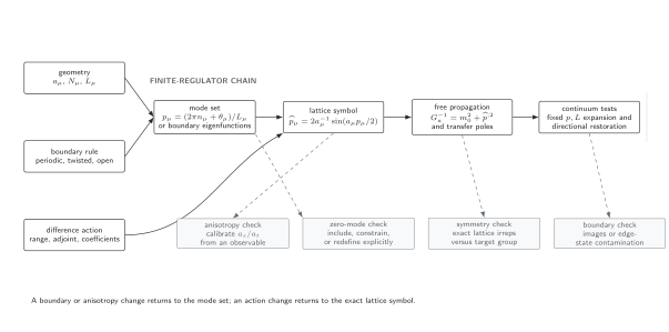
Geometry and action data jointly determine finite-regulator propagation. Periodic, twisted, open, and anisotropic choices cannot share one momentum or dispersion formula without translation. The continuum expansion is a tested limit, not an identification at finite spacing. The diagram is schematic and not to scale.

Common pitfalls

Using continuum momentum everywhere. $p_\mu$ labels the Fourier mode, while $\widehat p_\mu$ is the symbol of the chosen difference operator. Substituting one for the other changes the finite-regulator action.

Treating the Brillouin-zone boundary as a physical high-energy continuum state. Reciprocal periodicity identifies momentum labels modulo $2\pi/a$. Continuum interpretation is restricted to a controlled low-momentum region unless a different scaling limit is declared.

Fitting the wrong temporal image structure. Periodic time produces backward propagation. A single exponential is justified only in a window where the omitted image is below the declared tolerance.

Calling a removed zero mode harmless. A constraint on the mean field changes the measure. State it, and test whether the target observable becomes independent of that prescription in the intended limit.

Exercises

1. Green-function normalization. Starting from the momentum sum for $G_a(x-y)$, apply $-\Delta_a+m_0^2$ and derive $a^{-d}\delta_{x,y}$.

Solution

The operator multiplies each Fourier term by $K_a(p)$, canceling the denominator. Completeness then gives

$$\frac1V\sum_pe^{ip\cdot(x-y)} =\frac{\delta_{x,y}}{a^d}.$$

Any different factor signals an inconsistent transform pair.

2. Directional breaking. In two spatial dimensions compare $\widehat{\mathbf p}^2$ for $\mathbf p_1=(q,0)$ and $\mathbf p_2=(q/\sqrt2,q/\sqrt2)$ through $O(a^2)$.

Solution

Both have continuum norm $q^2$. The expansion gives

$$\widehat{\mathbf p}_1^2=q^2-\frac{a^2q^4}{12}+O(a^4), \qquad \widehat{\mathbf p}_2^2=q^2-\frac{a^2q^4}{24}+O(a^4).$$

Their difference $-a^2q^4/24+O(a^4)$ is a finite-spacing rotational-symmetry diagnostic.

What you can now do

You should now be able to normalize and invert a finite lattice kernel, derive its exact transfer dispersion, and separate zero-mode, finite-volume, and cutoff effects using independent tests. Continue with Exact Symmetries, Broken Spacetime Symmetries, and Restoration to turn directional cutoff effects and exact lattice transformations into a systematic restoration program.

References

• Montvay, István, and Gernot Münster. Quantum Fields on a Lattice. Cambridge University Press, 1994, chs. 1–2. doi:10.1017/CBO9780511470783.

Further reading

• Rothe, Heinz J. Lattice Gauge Theories: An Introduction. 4th ed. World Scientific, 2012, §§2.1–2.3. doi:10.1142/8229.
• Smit, Jan. Introduction to Quantum Fields on a Lattice. Cambridge University Press, 2002, chs. 2–3. doi:10.1017/CBO9780511583971.