Physical Gauge Hilbert Spaces and Constraint Enforcement

The tensor product of link and matter Hilbert spaces contains redundant gauge copies and states that violate Gauss’s law. Physical gauge states lie in a declared charge sector of all local generators. One may construct an invariant basis, apply a group-averaging projector, eliminate redundant variables, or suppress violations energetically, but these methods have different inner products, boundary-sector behavior, and error guarantees.

Required background. Lattice gauge Hamiltonians and Gauss’s law define the constraint algebra; local Hilbert-space regulators define the finite representation being constrained.

Helpful background. Constrained reduction distinguishes reduction from gauge fixing, while representations and intertwiners supply invariant-vertex bases.

Kernel and group-average constructions

Constraint and projector card. For a compact connected Lie group, the singlet sector is the simultaneous kernel of all $G_x^a$ ; charged sectors carry declared local irreducible representations. Haar measure on the full vertex group $G^V$ is normalized, and a non-Abelian character projector includes the irrep dimension. Do not drop a vertex average by importing the Abelian one-relation rule: determine the actual kernel of the group action, including boundary and common-center data.

For an Abelian constraint, or for a chosen mutually commuting set of charge operators $G_x$ with prescribed eigenvalues $q_x$ , define

\mathcal H_{\mathrm{phys},q}= \bigcap_x\ker(G_x-q_x).

For a non-Abelian singlet sector, the corresponding definition is the simultaneous kernel of every Lie-algebra generator $G_x^a$ ; a charged boundary or matter sector must instead declare the local irreducible representations it carries. Let $q_x$ label such an irrep, with dimension $d_{q_x}$ and character $\chi_{q_x}$ . Normalized Haar averaging gives the central projector onto the product isotypic sector,

P_{\boldsymbol q} =\left(\prod_x d_{q_x}\right) \int_{G^V}\!\prod_x\mathrm dg_x\, \left[\prod_x\chi_{q_x}(g_x)^*\right]U(\boldsymbol g).

For a singlet or an Abelian sector, every $d_{q_x}=1$ . In a finite group, the integral becomes a normalized finite sum. The dimension factor is required by character orthogonality: omitting it gives the right image but not an idempotent projector for $d_{q_x}>1$ . A character projects onto the entire non-Abelian isotypic component; selecting explicit multiplet indices requires matrix-element projectors or intertwiners. Verify

P_{\boldsymbol q}^\dagger=P_{\boldsymbol q},\qquad P_{\boldsymbol q}^2=P_{\boldsymbol q}, \qquad [P_{\boldsymbol q},H]=0.

This construction implements the Gauss sectors of the canonical lattice Hamiltonian Kogut and Susskind 1975, pp. 395–408.

Constraint redundancies depend on the group, matter content, and boundary conditions. In pure $\mathbb Z_2$ gauge theory on a closed connected graph, the product of all star operators is the identity, so only $V-1$ star constraints are independent. The product of individually normalized commuting star projectors is nevertheless still idempotent; the redundancy matters when counting sectors or dividing by gauge-orbit size. For a non-Abelian group, a common transformation generally conjugates every link and is not the identity; only the kernel of the actual group action, such as common central elements in a pure-link representation, is redundant. Determine that kernel rather than automatically dropping one vertex factor.

An invariant basis couples the representation indices meeting at each vertex through intertwiners. It removes unphysical states before computation and makes exact constraint preservation automatic, but can introduce nonlocal recoupling data and complicated operators. Independent-loop descriptions and their residual relations are discussed by Loll 1993, pp. 224–227.

Independent state counting on a small graph

Consider pure $\mathbb Z_2$ gauge theory on a connected open graph with $E$ links and $V$ vertices. The redundant tensor product has dimension $2^E$ . There are $V-1$ independent star constraints because the product of all stars is the identity. Therefore

\dim\mathcal H_{\mathrm{phys}}=2^{E-(V-1)}.

For the two-plaquette open rectangle with $E=7$ and $V=6$ , this gives $2^{7-5}=4$ . The two independent remaining binary variables can be chosen as plaquette fluxes. Direct projector rank, orbit counting, and cycle-space counting must all agree. This is a stronger check than observing $\langle G_x\rangle\simeq1$ in a few states.

Boundary charges change the count. Fixing external endpoints or allowing electric flux through the boundary changes which star constraints are imposed and which sectors are summed. State the boundary Hilbert space before comparing dimensions.

Penalties, postselection, and leakage

A penalty Hamiltonian

H_\lambda=H+\lambda C, \qquad C=\sum_x(G_x-q_x)^2

raises unphysical sectors when $[H,C]=0$ . If the smallest nonzero eigenvalue of $C$ is $c_{\min}$ , the unphysical weight of any normalized state satisfies

1-\langle P_{\boldsymbol q}\rangle\le\frac{\langle C\rangle}{c_{\min}}.

This converts a measured constraint residual into an interpretable bound. Finite $\lambda$ still allows unphysical eigenstates and can distort time scales; if an approximate evolution does not commute with $C$ , leakage can grow dynamically.

Postselection discards outcomes outside the accepted sector. Report the acceptance probability and any correlation between acceptance and the measured observable. Error mitigation that extrapolates in a penalty or noise parameter remains model dependent and is not exact projection.

The shared map marks this distinction at the point where the branches rejoin.

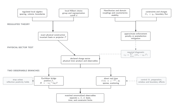
A regulated Hamiltonian and local Hilbert space feed exact constraints or penalty suppression, then a physical sector; a positive transfer-matrix branch and a direct real-time branch meet only at matched renormalized continuum observables, with leakage and positivity failures marked.

Invariant bases and projectors enter the declared charge sector exactly. Penalties and postselection reach it only conditionally and require a quantitative leakage or acceptance diagnostic before an observable is called physical. The diagram is schematic.

Gauge fixing versus physical reduction

Fixing a maximal tree can remove redundant link variables on a finite graph, leaving loop variables and boundary degrees of freedom. The Jacobian, residual global transformations, and topology must be retained. A gauge-fixed coordinate representation can be isomorphic to the physical Hilbert space, but simply setting links to the identity without transforming states and operators is not a projection.

For non-Abelian theories, Mandelstam relations and intertwiner multiplicities make loop bases overcomplete unless independent constraints are resolved. Whichever basis is chosen, verify the physical inner product and matrix elements against projector calculations on a small graph.

Adversarial failure case

On a pure $SU(2)$ graph, suppose one deletes an entire vertex average by assuming that the product of local transformations is redundant as in closed $\mathbb Z_2$ theory. A common noncentral rotation conjugates every link and is not the identity, so the reduced average admits globally nonsinglet states; for the full link representation on a connected graph, the kernel is the common center. Such a state may still have $\langle G_x^a\rangle=0$ by symmetry while its quadratic Casimir residual is nonzero. Act with a common noncentral group element, compare the reduced and full projector ranks, and match their images against an intertwiner basis to reveal the spurious sector. Idempotence alone cannot do so: normalized averaging over the remaining subgroup is still a projector.

Observable-level validation

Verify $P^\dagger=P$ , $P^2=P$ , and $[P,H]=0$ numerically or algebraically on a complete small-graph basis.
Compare the projector rank with independent orbit, cycle-space, or intertwiner counting in every boundary-charge sector.
Determine the group-action kernel by acting with common central and noncentral transformations; do not infer it from the Abelian case.
Measure squared Gauss or Casimir residuals and the full sector distribution, not only linear generator expectations.
For penalties or postselection, report leakage or projector weight, acceptance probability, and the shift of at least one physical matrix element as the enforcement parameter changes.

Common pitfalls

Checking only $\langle G_x-q_x\rangle$ . Positive and negative violations can cancel. Use $\langle(G_x-q_x)^2\rangle$ , projector weight, or the full sector distribution.

Forgetting boundary flux. A charged state in a region requires matter charge, boundary electric flux, or both. Imposing a neutral closed-lattice constraint can erase the intended sector.

Treating every constraint as independent. Naively subtracting one binary degree of freedom for every $\mathbb Z_2$ star gives the wrong state dimension because the product of all stars is the identity. Identify relations and the kernel of the group action before counting; a product of individually normalized commuting projectors remains well defined even when one constraint follows from the others.

Learning outcomes

Construct a normalized projector or invariant basis for a small gauge graph and verify its idempotence, rank, boundary sector, and physical inner product by an independent state count.
Given constraint-enforcement data, distinguish exact projection, energetic suppression, postselection, and a false zero from an undersensitive linear diagnostic using projector weight and squared residuals.

Exercises

Derive the physical dimension for a connected pure $\mathbb Z_2$ graph with cycle rank $b_1=E-V+1$ .

Solution

There are $V-1$ independent star constraints, so the dimension is $2^{E-V+1}=2^{b_1}$ , one binary degree of freedom per independent cycle.

A state has $\langle C\rangle=3\times10^{-4}$ and $c_{\min}=1$ . Bound its unphysical weight.

References

Section titled “References”- Kogut, J. B., and Susskind, L. (1975). Hamiltonian formulation of Wilson’s lattice gauge theories. Physical Review D, 11, 395–408. DOI.
- Loll, R. (1993). Lattice gauge theory in terms of independent Wilson loops. Nuclear Physics B Proceedings Supplements, 30, 224–227. DOI.
Further reading
Section titled “Further reading”- Zohar, E., Cirac, J. I., and Reznik, B. (2016). Quantum simulations of lattice gauge theories using ultracold atoms in optical lattices. Reports on Progress in Physics, 79, 014401. DOI.
Original QFT.org content:CC BY 4.0, unless an item supplies different terms. Third-party material retains its own terms.