Reflection Positivity and Transfer-Matrix Criteria

A Euclidean lattice measure supports a positive-state transfer interpretation when it is reflection positive with respect to a declared time reflection and satisfies the additional regularity and translation assumptions needed for reconstruction. For the nearest-neighbor scalar, the one-time-step kernel factors into positive multiplication operators and a positive Gaussian convolution, producing a positive self-adjoint transfer operator. Spatial improvement is often compatible with this construction; extended couplings across the reflection plane in Euclidean time can spoil it, producing negative spectral weights or extra unphysical poles even when the small-momentum dispersion looks improved.

Required background. Scalar Lattice Actions and Difference Operators supplies the quadratic action and boundary-sensitive adjoints. Reflection Positivity within Osterwalder–Schrader Reconstruction defines the foundational positivity condition and its reconstruction role.

Helpful background. Self-Adjointness, Extensions, and Unitary Evolution explains why positivity and self-adjointness are operator-domain statements.

Time reflection and the positive-time algebra

Choose a distinguished Euclidean-time coordinate $t=na_t$. A link reflection about the plane between slices $0$ and $1$ acts on sites by

$$\vartheta(t,\mathbf x)=(a_t-t,\mathbf x).$$

For real scalar fields, define the antilinear action on a functional $F$ by

$$(\Theta F)[\phi]=F[\phi\circ\vartheta]^*.$$

Let $\mathcal A_+$ be an algebra of bounded cylindrical functionals, together with polynomial cylinder functionals whose required moments exist, supported strictly on the positive-time half-lattice. Reflection positivity is the inequality

$$\langle(\Theta F)F\rangle_E\ge0 \qquad\text{for every }F\in\mathcal A_+.$$

The support restriction matters: positivity of ordinary expectation values, positivity of the Boltzmann weight, and positivity of a covariance matrix are not substitutes for this reflected quadratic form. Site reflection and link reflection lead to related but not identical factorizations, especially when interactions or gauge links lie on the reflection plane.

Reflection and regulator conventions. We use a flat Euclidean lattice, real scalar fields, link reflection in the distinguished time direction, and the weight $e^{-S_E}$. The site-wide conventions apply. The reflection plane, allocation of variables on that plane, temporal boundary condition, and support algebra are local data. “Positive transfer matrix” means a positive self-adjoint operator on the Hilbert space reconstructed from the finite lattice; that Hilbert space need not be finite-dimensional when site fields are continuous. It is not a proof of the full continuum Wightman theory.

Reflection positivity turns $\mathcal A_+$ into a pre-Hilbert space with sesquilinear form

$$(F,G)_{\mathrm{OS}} =\langle(\Theta F)G\rangle_E.$$

One quotients null vectors and completes. A one-step positive-time translation then induces a contraction that can be represented, under suitable assumptions, by a transfer operator $T$. If $T$ is positive, self-adjoint, and injective, spectral calculus defines $H=-a_t^{-1}\log T$; after normalizing the vacuum energy, $T=e^{-a_tH}$ with $H\ge0$. If $T$ has a kernel, the logarithm requires a support/domain qualification. The full reconstruction requires more than this single inequality. The Euclidean axioms and reconstruction hypotheses are developed in Osterwalder and Schrader 1973, pp. 83–112; Osterwalder and Schrader 1975, pp. 281–305 corrects the original lemma and supplies stronger sufficient growth conditions.

One-step kernel for the nearest-neighbor scalar

Keep space discretized and collect all scalar values on time slice $n$ into a vector $\varphi_n$. Write the action as

$$S_E=\sum_n\left[ \frac{a_s^{d-1}}{2a_t} \lVert\varphi_{n+1}-\varphi_n\rVert^2 +\frac{a_t}{2}\bigl(U(\varphi_{n+1})+U(\varphi_n)\bigr) \right],$$

where

$$U(\varphi)=a_s^{d-1}\sum_{\mathbf x}\left[ \frac12\sum_i(\nabla_i^+\varphi_{\mathbf x})^2 +\frac12m_0^2\varphi_{\mathbf x}^2 +V_{\mathrm{int}}(\varphi_{\mathbf x}) \right].$$

The symmetric split assigns half of the within-slice potential to each adjacent step. The transfer kernel is

$$T(\varphi',\varphi) =\mathcal N \exp\!\left[ -\frac{a_s^{d-1}}{2a_t}\lVert\varphi'-\varphi\rVert^2 -\frac{a_t}{2}U(\varphi') -\frac{a_t}{2}U(\varphi) \right].$$

Symmetry under $\varphi\leftrightarrow\varphi'$ makes the integral operator self-adjoint with the flat slice measure, assuming $U$ is real, stable enough for the measure to exist, and the kernel defines a bounded operator or closed quadratic form on a stated domain. Positivity is stronger than the pointwise statement $T(\varphi',\varphi)>0$. Factorize

$$T=M_{e^{-a_tU/2}}\,C\,M_{e^{-a_tU/2}},$$

where $M$ is multiplication and $C$ is Gaussian convolution. Let $N_{\mathrm{slice}}$ be the number of real field variables on one time slice. For any square-integrable wavefunctional $\Psi$,

$$\langle\Psi,C\Psi\rangle =\int\frac{\mathrm d^{N_{\mathrm{slice}}}\pi}{(2\pi)^{N_{\mathrm{slice}}}} \widetilde c(\pi)\, \lvert\widetilde\Psi(\pi)\rvert^2\ge0,$$

because the Fourier transform of the Gaussian, $\widetilde c(\pi)$, is nonnegative. Hence $C\ge0$ and $T\ge0$. This finite-slice factorization is the minimal analytic benchmark. A real stable action, nearest-neighbor temporal difference, symmetric potential allocation, and positive slice measure are sufficient for this simple flat-measure construction; other reflection-positive formulations can use different factorizations.

For one spatial site with $U(\varphi)=m_0^2\varphi^2/2$ and $m_0^2>0$, the kernel is Gaussian and diagonalization recovers a lattice harmonic oscillator. Its energy gap $E_a$ satisfies

$$4\sinh^2\!\left(\frac{a_tE_a}{2}\right)=a_t^2m_0^2,$$

the zero-spatial-momentum case of the cutoff dispersion derived on the propagator page. Agreement between kernel diagonalization and the propagator pole is an independent normalization check. At $m_0=0$, the noncompact constant mode has no normalizable vacuum.

Positive spectral weights

If $T=e^{-a_tH}$ acts on a positive Hilbert space, the temporal extent is infinite, and $\mathcal O$ corresponds to an operator on a time slice, then for integer $n>0$

$$C(n a_t) =\langle0|\mathcal O,T^n\mathcal O^\dagger|0\rangle =\int_0^\infty e^{-n a_tE}\,\mathrm d\rho_{\mathcal O}(E), \qquad \mathrm d\rho_{\mathcal O}(E)\ge0.$$

Here $E$ is the excitation gap above the vacuum energy $E_0$, and $\rho_{\mathcal O}$ is the positive spectral measure generated by $\mathcal O^\dagger|0\rangle$. If $\mathcal O$ overlaps the vacuum, the measure contains a contribution at $E=0$; subtract that contribution before interpreting a nonzero lowest gap.

For a discrete spectrum, the integral becomes

$$\sum_k \lvert\langle k|\mathcal O^\dagger|0\rangle\rvert^2 e^{-n a_t(E_k-E_0)}.$$

Every spectral weight is nonnegative. This implies useful diagnostics:

• the adjoint-paired correlator $\langle0|\mathcal O T^n\mathcal O^\dagger|0\rangle$ is nonnegative for any $\mathcal O$ in the stated domain;
• when $C_n=C(na_t)>0$, define $E_{\mathrm{eff}}(n)=a_t^{-1}\log(C_n/C_{n+1})$. Log-convexity gives $E_{\mathrm{eff}}(n+1)\le E_{\mathrm{eff}}(n)$ and $E_{\mathrm{eff}}(n)\ge E_1$, where $E_1=\inf\operatorname{supp}\rho_{\mathcal O}$ after any vacuum term is removed, so the effective energy approaches the lowest contributing gap from above; and
• reflected Gram matrices are positive semidefinite. For link reflection $\vartheta(n)=1-n$, slices $n_i,n_j\ge1$ give entries $C((n_i+n_j-1)a_t)$; equivalently, if times are measured from the reflection plane at $a_t/2$, this is the Hankel form $C(t_i+t_j)$.

These consequences depend on the operator and reflection assignment. Gauge-variant fields, fermionic insertions, derivative operators odd under reflection, and subtracted correlators require the corresponding conjugation and sign structure; testing scalar positivity formulas on them is invalid. At finite periodic temporal extent, backward propagation produces a cosh-like form, so the simple log-ratio monotonicity statement must be replaced by its finite-$T$ version.

The relationship among Euclidean reflection, transfer evolution, the physical constraint space, and later Hamiltonian limits is summarized below. Inspect where positivity enters and where Gauss-law or local-Hilbert restrictions add separate conditions.

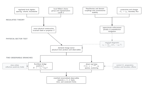
Exact and approximate constraint constructions share the same regulated inputs, but the approximate route must pass a volume-aware leakage test before its states are called physical. The Euclidean branch requires reflection positivity before a positive, self-adjoint transfer operator is claimed; the direct real-time branch instead requires controlled preparation, time step, observation window, and boundaries. Both still require matched observables and separate regulator limits. Schematic, not to scale.

Read the two lower branches as gated alternatives. Exact and approximate constraint enforcement use the same regulated algebra, Hilbert representation, Hamiltonian, and charge data; an approximate construction enters the declared sector only after a quantitative leakage test. The Euclidean branch then requires reflection positivity before a positive transfer claim, while the real-time branch requires its preparation, time-step, time-window, and boundary controls.

How an apparently improved action can fail

Suppose a temporal kinetic term includes next-nearest slices to cancel an $O(a_t^2)$ dispersion error. Its Fourier kernel may have the form

$$K(p_0)=m^2+c_1\bigl(1-\cos(a_tp_0)\bigr) +c_2\bigl(1-\cos(2a_tp_0)\bigr).$$

Appropriate $c_1,c_2$ can improve the small-$p_0$ expansion. Yet the cross-reflection part now couples more than one pair of slices. Loss of the simple one-slice factorization does not alone prove failure—an enlarged transfer construction may exist—but positivity must be re-established. For continuum-improved lattice gauge actions, the resulting transfer matrix can have complex eigenvalues and correlation functions can contain negative spectral weights Lüscher and Weisz 1984, p. 349. A smaller leading Taylor coefficient is therefore insufficient evidence for a positive spectral theory.

One can expose the failure without attempting full reconstruction:

1. write $S_E=S_++\Theta S_++S_{\mathrm{cross}}$ and test whether $e^{-S_{\mathrm{cross}}}$ lies in the reflection-positive cone; a common sufficient form is $-S_{\mathrm{cross}}=\sum_\alpha c_\alpha(\Theta B_\alpha)B_\alpha$ with $c_\alpha\ge0$ and $B_\alpha\in\mathcal A_+$ supported on the declared positive-time half-lattice, as in the lattice construction of Osterwalder and Seiler 1978, §§2–3;
2. locate every pole of the free propagator in the complex energy plane;
3. decompose the time correlator into exponentials and inspect the signs and reality of residues; and
4. test reflected Gram matrices on a finite basis of positive-time functionals.

Passing a finite basis is necessary but not sufficient for the universal inequality. Failing one basis element is decisive.

Gauge actions have their own reflection assignments for oriented links and plaquettes. Wilson’s plaquette action admits a positive transfer construction under standard conditions Lüscher 1977, pp. 283–292 and Osterwalder and Seiler 1978, §§2–3, while arbitrary extended loops require renewed analysis. The explicit gauge Hamiltonian and Gauss-law projection belong to Transfer Matrices between Euclidean and Hamiltonian QFT.

What the criterion does not prove

Reflection positivity at fixed $a$ does not by itself prove:

• existence of an infinite-volume limit;
• existence or uniqueness of a continuum limit;
• restoration of Lorentz symmetry;
• locality and positivity of a proposed improved continuum observable;
• equivalence of Euclidean and Hamiltonian regulators after independent truncations; or
• the full hypotheses of a constructive reconstruction theorem.

Conversely, a finite-$a$ action that violates reflection positivity may still approach a unitary continuum theory if the violating states remain at the cutoff and decouple, a possibility analyzed for improved actions by Lüscher and Weisz 1984, §6, pp. 359–360. That is a stronger continuum claim: it requires explicit scale separation and positive renormalized observables across several spacings. One should not call the finite regulator positive while making that argument.

Reflection positivity controls one logical step, whereas the target statement also depends on cutoff, volume, and reconstruction limits. The diagram below keeps those axes separate; inspect the crossed routes before treating a positive finite-spacing kernel as a completed continuum construction.

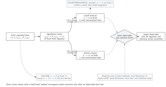
Both main routes apply cutoff removal and infinite volume while matching the target data before their results are compared. A broken phase and the periodic massless scalar give genuine order tests; $a\to0$ at fixed site count is instead a misidentified path because the box shrinks. Other truncation and time-evolution axes need their own declared schedules. The diagram is schematic and not to scale.

Observable-level validation checklist

Before claiming a transfer interpretation, verify:

• the reflection plane, positive-time algebra, conjugation, and boundary conditions are explicit;
• the action and measure are invariant under the reflection;
• the cross-plane couplings admit a nonnegative factorization or an applicable theorem;
• the one-step kernel is self-adjoint and positive as an operator, not merely pointwise;
• free poles have real nonnegative energies and the expected residue signs;
• reflected Gram matrices pass analytic and numerical tests;
• temporal improvement and extended loops have been checked separately from spatial improvement;
• the claimed spectral weights use operators with the correct reflection parity; and
• continuum conclusions are stated only after volume, tuning, symmetry, and cutoff limits are controlled.

Exercises

1. Positive Gaussian convolution. Let $(C\Psi)(x)=\int\mathrm dy\,e^{-\alpha(x-y)^2}\Psi(y)$ with $\alpha>0$. Show that $C$ is a positive operator.

Solution

Fourier transformation gives $\widetilde{C\Psi}(k)=\sqrt{\pi/\alpha}\,e^{-k^2/(4\alpha)}\widetilde\Psi(k)$. Plancherel’s identity then yields

$$\langle\Psi,C\Psi\rangle =\int\frac{\mathrm dk}{2\pi} \sqrt{\frac\pi\alpha} e^{-k^2/(4\alpha)} \lvert\widetilde\Psi(k)\rvert^2\ge0.$$

Multiplication on both sides by a real positive function preserves positivity, establishing the factorized transfer-kernel result.

2. A reflected Gram test. If $C(n)=A e^{-na_tE_1}+B e^{-na_tE_2}$ with $E_2>E_1>0$ and $A>0$, form the direct link-reflection matrix $M_{ij}=C(i+j-1)$ for $i,j=1,2$. Show that $A,B\ge0$ imply $M\ge0$ and explain how $B<0$ can be detected.

Solution

Write $M=A e^{-a_tE_1}v_1v_1^{\mathsf T}+B e^{-a_tE_2}v_2v_2^{\mathsf T}$ with $v_k=(1,e^{-a_tE_k})$. Nonnegative $A,B$ make it a sum of positive rank-one matrices. If $B<0$, the determinant is

$$\det M=AB\,e^{-a_t(E_1+E_2)} \bigl(e^{-a_tE_1}-e^{-a_tE_2}\bigr)^2<0,$$

so one eigenvalue is negative.

What you can now do

You should now be able to state the lattice reflection-positivity inequality, construct the nearest-neighbor scalar transfer kernel, and distinguish a positive finite-regulator interpretation from a full reconstruction or continuum claim. Continue with Bare Parameters, Tuning Conditions, and Continuum Targets to specify which physical theory a sequence of such regulated transfer systems is meant to approach.

References

• Lüscher, Martin. “Construction of a Selfadjoint, Strictly Positive Transfer Matrix for Euclidean Lattice Gauge Theories.” Communications in Mathematical Physics 54, no. 3 (1977): 283–292. doi:10.1007/BF01614090.
• Lüscher, Martin, and Peter Weisz. “Definition and General Properties of the Transfer Matrix in Continuum Limit Improved Lattice Gauge Theories.” Nuclear Physics B 240, no. 3 (1984): 349–361. doi:10.1016/0550-3213(84)90270-0.
• Osterwalder, Konrad, and Robert Schrader. “Axioms for Euclidean Green’s Functions.” Communications in Mathematical Physics 31, no. 2 (1973): 83–112. doi:10.1007/BF01645738.
• Osterwalder, Konrad, and Robert Schrader. “Axioms for Euclidean Green’s Functions II.” Communications in Mathematical Physics 42, no. 3 (1975): 281–305. doi:10.1007/BF01608978.
• Osterwalder, Konrad, and Erhard Seiler. “Gauge Field Theories on a Lattice.” Annals of Physics 110, no. 2 (1978): 440–471. doi:10.1016/0003-4916(78)90039-8.