

Spectra from Euclidean Correlation Matrices
A matrix of Euclidean correlators isolates several finite-volume levels by resolving their different overlap vectors, not by fitting many exponentials to one correlator without constraint. The generalized eigenvalue problem (GEVP) turns an operator basis into principal correlators whose asymptotic slopes approach energies. Reliability requires a declared finite-volume symmetry sector, a positive and well-conditioned metric matrix, correlated uncertainty propagation, and stability against basis removal, reference-time choice, fit window, and deliberately omitted states.
Required background. Operator Bases, Effective Masses, and Excited-State Control supplies single-correlator spectral fitting and basis design. Estimators, Covariance, and Resampling supplies the correlated estimators used below.
Helpful background. Spectral Decomposition of Two-Point Functions supplies the Hilbert-space origin of the exponentials.
Correlation matrices in one finite-volume sector
Section titled “Correlation matrices in one finite-volume sector”Choose operators projected to the same total momentum , lattice irrep and row , internal quantum numbers, and boundary conditions. With unit-normalized finite-volume eigenstates, , define
Any or volume factor used in another source is absorbed here into ; it must be restored before comparing overlaps.
Spectral-extraction convention. The correlator matrix, metric, and fitted levels all belong to one declared finite-volume symmetry sector, with unit-normalized eigenstates and temporal wrapping included whenever the fit window can resolve it.
The detailed choices are:
| Field | Choice used on this page |
|---|---|
| State norm | |
| Operator projection | Every has identical , , flavor and other exact quantum numbers; different constructions may have different overlaps |
| Time behavior | Forward exponentials are displayed; backward and thermal-wrap terms are included in fits when approaches |
| Matrix metric | is Hermitian positive definite after a declared numerical rank cut; whitening uses that retained subspace |
| Uncertainty | The same blocked bootstrap or jackknife sample builds , solves the GEVP, fits levels, and passes them downstream |
| Output | Energies and overlap vectors are finite-volume quantities; no phase shift is assigned on this page |
Multi-hadron operators must span the relevant momentum partitions and single-hadron-like constructions. A basis containing only local operators can have exponentially or parametrically small overlap with spatially extended two-particle states; a clean plateau then demonstrates isolation within the seen subspace, not completeness of the spectrum.
The generalized eigenvalue problem
Section titled “The generalized eigenvalue problem”For , solve
Numerically, diagonalize , retain eigenmodes satisfying a predeclared condition-number or noise criterion, and form the whitened matrix
It is Hermitian in exact arithmetic and has the same generalized eigenvalues. The principal effective energy
approaches only after contamination from states outside the resolved subspace is controlled. Under the hypotheses analyzed by Blossier and collaborators, choosing makes the leading omitted-state correction to the effective energy scale as rather than with an arbitrary “gap” (Blossier et al. 2009, §§ 2–3). The theorem does not say that increasing cures a singular basis or exponentially growing noise.
Eigenvector labels can swap near avoided crossings. Track levels using a combination of energy continuity and normalized overlaps, for example
An energy ordering alone is not a quantum-number assignment.
Exact two-state benchmark
Section titled “Exact two-state benchmark”Let two linearly independent operators couple to exactly two states:
Then
so the generalized eigenvalues are exactly , independent of the overlap matrix. This checks the normalization and explains the method: the GEVP cancels overlaps only when the resolved basis spans the contributing states.
Now add an omitted third state,
The correction depends on the direction of as well as the gap . If is nearly parallel to a retained overlap vector, one principal correlator may look stable while its energy is biased. This is why the synthetic missing-state challenge must vary overlap geometry, not just add a small exponential.
A reproducible extraction contract
Section titled “A reproducible extraction contract”- Build the sector. List every operator, momentum partition, smearing or displacement, irrep projection, and expected nearby noninteracting level.
- Estimate one covariance object. Preserve configuration or chain blocks across all ; symmetrize only through a documented estimator.
- Choose rank without looking at the answer. Declare the singular-value or conditioning criterion and repeat the analysis with adjacent ranks.
- Solve sample by sample. Recompute whitening, eigenvectors, level tracking, and fits in every resample; do not attach fixed eigenvectors to fluctuating matrices.
- Fit correlated principal correlators. Include backward terms and extra exponentials when the chosen window requires them.
- Challenge the basis. Remove each operator class in turn, vary and fit windows, and inject a synthetic state with an overlap direction designed to mimic a retained level.
- Freeze finite-volume outputs. Report , the covariance among all levels, overlap diagnostics, and unresolved ambiguities before any scattering fit.
The original variational construction and its lattice application are developed by Lüscher and Wolff 1990, §§ 2–3, pp. 226–239.
Adversarial failure. A basis with two nearly proportional operators gives an eigenvalue below the noise floor. Keeping it can create a wildly fluctuating whitened direction and a seemingly precise level after nonlinear sorting. Dropping it after inspecting which choice produces the desired energy is also biased. The rank rule must be fixed from conditioning and replicated under resampling before inspecting the downstream phase shift.
Two maps locate the output of this page. The first shows that covariance-aware state isolation is an inference from correlators; the second shows that the resulting finite-volume energies remain inputs to a branch-specific finite-to-infinite-volume relation.
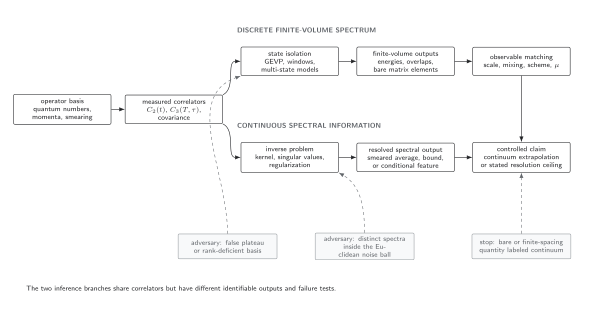
Two inference problems share the same regulated correlators. Discrete energies and overlaps, together with validated connected and disconnected three-point estimators, support bare matrix elements that require matching and continuum control before becoming physical results. Continuous reconstruction identifies only smeared averages, bounds, or conditional features at the demonstrated resolution; without separate matching and continuum analysis it ends at a methodological ceiling. Dashed boxes mark failure tests. The diagram is schematic and not to scale.
The next map begins at those extracted levels. Inspect the required short-range, branch, normalization, and covariance conditions before following an arrow toward an amplitude.
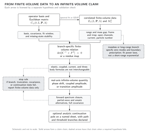
Finite-volume information reaches an infinite-volume claim only through a branch-specific map. Solid arrows show the controlled chain; dashed arrows show the long-range alternative and the stop rule. The image is schematic, not to scale, and the displayed determinant is structural: its channel, irrep, partial-wave, normalization, and sign conventions must be fixed locally.
Observable-level validation
Section titled “Observable-level validation”Accept a level only if:
- the operator basis contains the relevant single- and multi-particle momentum structures for its sector;
- is Hermitian within uncertainty and is positive on the retained subspace;
- energies are stable under removal of operator classes, adjacent rank cuts, , fit-window, and backward-term variations;
- eigenvector-overlap tracking resolves or explicitly reports near-degenerate label ambiguity;
- a synthetic omitted state with challenging overlaps is either recovered or produces a quoted bias; and
- the full cross-level covariance, not independent error bars, enters the quantization analysis.
What you can now do
Section titled “What you can now do”You can now (1) construct and solve a -normalized GEVP with finite-volume state and operator normalization explicit, and (2) demonstrate level stability quantitatively under basis reduction, reference-time and fit-window changes, and a synthetic missing-state challenge.
Elastic Two-Body Quantization Conditions converts controlled two-particle levels into a real-axis amplitude. Moving Frames, Cubic Irreducible Representations, and Partial-Wave Mixing supplies the irrep bookkeeping needed to interpret the operator sector.
Exercises
Section titled “Exercises”1. Basis invariance. Replace the operators by with . Show that the exact generalized eigenvalues are unchanged.
Solution
. The transformed GEVP is . Multiplying by and setting gives the original GEVP. Hence a nonsingular basis change preserves the exact spectrum, although finite-noise conditioning can change dramatically.
2. Missing-state scale. For , in common units, compare at and .
Solution
The factors are and . Doubling reduces this asymptotic contamination by a factor of eleven, but the calculation still needs a covariance and noise check; the exponential estimate alone is not an uncertainty.
References
Section titled “References”- Blossier, Benoît, Michele Della Morte, Georg von Hippel, Tereza Mendes, and Rainer Sommer. “On the Generalized Eigenvalue Method for Energies and Matrix Elements in Lattice Field Theory.” Journal of High Energy Physics 2009, no. 4 (2009): 094. DOI. Open PDF.
- Lüscher, Martin, and Ulli Wolff. “How to Calculate the Elastic Scattering Matrix in Two-Dimensional Quantum Field Theories by Numerical Simulation.” Nuclear Physics B 339 (1990): 222–252. DOI.
Original QFT.org content:CC BY 4.0, unless an item supplies different terms. Third-party material retains its own terms.