Real-Time Evolution and Observable Extraction

Real-time quantum simulation becomes a QFT calculation only when the measured estimator is tied to a renormalized response, spectral, scattering, number, flux, or inclusive observable. The protocol must specify the prepared state, time ordering, ancillary interference if used, finite-time and finite-volume windows, sampling cost, operator matching, and continuum conversion. A precise bit string is not yet a physical observable.

Required background. Digital Hamiltonian simulation and algorithmic error supplies the approximate unitary. Preparing interacting QFT states supplies certified input states. Real-time evolution, scattering, and observable extraction supplies the regulator-level observable definitions.

Helpful background. LSZ reduction: poles, residues, and stable external states supplies the continuum conditions for stable-particle scattering amplitudes.

Unequal-time observables

Convention and regulator card. At fixed $(a,L,d_{\rm loc})$, let $H$ be the matched regulated Hamiltonian, $O_R=Z_O(a)O_{\rm bare}+\sum_jc_j(a)O_j$ the matched operator, and $U(t)=e^{-iHt}$. Time is Minkowski time. The measurement window $0\le t\le T$, boundary-reflection time, state sector, and operator normalization are declared before data are taken.

For a stationary state $\rho$, an unequal-time correlator is

$$C_{AB}(t)=\operatorname{Tr}\!\left[\rho\,A(t)B(0)\right], \qquad A(t)=U^\dagger(t)AU(t).$$

If $A$ and $B$ are unitary or decomposed into measurable unitaries, an ancilla interference experiment can encode the real and imaginary parts of $C_{AB}$ in complementary ancilla observables. Every controlled operation, coefficient, and reconstruction covariance belongs to the estimator definition. Direct projective measurements of local densities may be simpler, while nonunitary field operators require a linear-combination or dilation construction.

The retarded response

$$G^R_{AB}(t)=-i\theta(t)\langle[A(t),B(0)]\rangle$$

requires both orderings or an equivalent response protocol. A finite transform

$$\widetilde G_T(\omega)=\int_0^T\mathrm dt\,w(t)e^{i\omega t}G^R(t)$$

is the exact transform of a windowed signal. Its resolution is $O(1/T)$, and the choice of window $w(t)$ changes line shapes. Zero-padding does not create spectral resolution.

Scattering, flux, and inclusive estimators

A wave-packet scattering calculation prepares separated incoming packets, evolves through an interaction window, and measures outgoing particle content or flux before boundary reflections return. The packet definitions, vacuum subtraction, wave-function renormalization, and finite-volume normalization are part of the observable. The constructive scalar-field algorithm of Jordan, Lee, and Preskill 2014, §§ 2–4 illustrates this sequence and its separate preparation, evolution, and detection errors.

At finite regulator, a detector region $R_{\rm out}$ might use an integrated number or current estimator

$$N_{R}(t)=\sum_{x\in R_{\rm out}}a^d\,n_x(t), \qquad \Phi_R=\int_{t_1}^{t_2}\mathrm dt\sum_{x\in\partial R}a^{d-1}j_x(t).$$

The continuity equation supplies a strong check: the change of charge inside $R$ should agree with the boundary flux up to discretization, boundary, compilation, and measurement errors.

Inclusive observables can avoid reconstructing every exclusive final state by measuring a projector, response function, or suitably integrated current. Amplitude estimation can change the dependence on a sampling tolerance under coherent-oracle assumptions, but the state-preparation and reflection oracles, coherent depth, and final confidence must be counted. Ordinary shot sampling remains $O(\sigma_O^2/\epsilon_{\rm stat}^2)$ for variance $\sigma_O^2$.

Measurement in the shared flow

The figure’s final solid arrow is not simply “readout”: it maps an encoded operator and finite-time experiment back to a regulated QFT estimator. Inspect the dashed exact-correlator and continuum-matching checks.

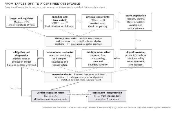
Measurement closes the finite-regulator part of the simulation chain. Ancilla interference, direct densities, fluxes, or inclusive projectors produce encoded estimators; operator renormalization, time-window response, boundary checks, and exact small-system correlators connect them to QFT observables. The map is schematic, not a circuit prescription.

The minimum claim–resource–evidence record requires the observable, its estimator, sampling cost, matching, and verification to refer to the same target accuracy.

Analytic benchmark: free scalar correlator

For the free periodic chain in its vacuum, use $[\phi_x,\pi_y]=i\delta_{xy}/a$ and a unitary site Fourier transform. Then

$$C(t,x)=\langle\phi_x(t)\phi_0(0)\rangle =\frac1N\sum_k\frac{e^{ikx-i\omega_kt}}{2a\omega_k},$$

with $\omega_k^2=m_0^2+4a^{-2}\sin^2(ka/2)$. At $t=0$, $C(0,x)$ is real and even in $x$; $C(-t,x)=C(t,x)^*$; and every temporal Fourier peak lies at a known $\omega_k$. These symmetry and spectral checks diagnose phase, normalization, and time-order errors.

For a small interacting chain, exact diagonalization gives

$$C(t)=\sum_n e^{-i(E_n-E_0)t} |\langle n|\phi|0\rangle|^2.$$

Freeze several early times for tuning and reserve later times plus a second operator as held-out tests. Vary $T$, the window, packet separation, and $L$ separately. A continuum conversion is attempted only after $Z_O(a)$ and the line of constant physics are supplied by the regulator formulation.

Adversarial failures

Longer transform, reflected signal. Increasing $T$ sharpens Fourier bins but includes a boundary echo. Vary $L$ and require the extracted feature to stabilize inside a pre-reflection window.

Bare operator called physical. The encoded lattice field is measured accurately, but its normalization and mixing are omitted. The result is a bare correlator, not the renormalized continuum quantity.

Ancilla phase convention reversed. Real and imaginary parts are interchanged or signed incorrectly while $|C(t)|$ looks plausible. Check $C(0)$, Hermiticity, and the exactly solvable free phase.

Packet detector counts vacuum fluctuations. A local occupation proxy has a nonzero vacuum expectation. Measure and subtract the same regulated vacuum, with covariance propagated.

Observable-level validation checklist

• Define the renormalized observable, encoded decomposition, state, time ordering, normalization, and physical units.
• Include preparation, controlled evolution, ancilla or direct measurement, reconstruction, and sampling in one protocol.
• Check equal-time normalization, Hermiticity, conservation or Ward identities, and an exact small-system time series.
• Vary time window, spatial volume, packet width and separation, detector region, and local dimension independently.
• Propagate covariance from vacuum subtraction, linear-combination reconstruction, and shared circuit samples.
• State the conversion from finite-regulator estimator to continuum quantity and stop before any unsupported scattering or spectral interpretation.

Exercises

1. Finite-time resolution

A correlator is trusted only through $T=40/m$. Estimate the smallest resolvable angular-frequency separation and explain why zero-padding cannot improve it.

Solution

The natural separation is of order $2\pi/T\simeq0.157m$ (window-dependent constants can differ). Zero-padding samples the same finite-time transform more densely; it does not add information beyond $T$.

2. Sampling an inclusive projector

For a projector $P$, $p=\langle P\rangle=0.2$. How many independent shots suffice for a standard error at most $0.01$?

Solution

The Bernoulli variance is $p(1-p)=0.16$. Require $\sqrt{0.16/N}\le0.01$, so $N\ge1600$. Preparation failures and correlated shots would increase the required raw count.

Learning outcomes

After working this page, you should be able to:

• Design an end-to-end protocol for a renormalized unequal-time, response, scattering, flux, spectral, or inclusive observable, including state preparation, evolution, operator decomposition, sampling, and continuum conversion.
• Select time, volume, wave-packet, detector, and Fourier windows that separate physical signal from transients, periodic reflections, digitization, and measurement reconstruction error.

Handoff

Verification, error mitigation, and observable certification builds independent evidence for the resulting estimator. Resource and continuum certification propagates its target precision through regulator and logical-resource choices.

References

• Jordan, Stephen P., Keith S. M. Lee, and John Preskill. “Quantum Computation of Scattering in Scalar Quantum Field Theories.” Quantum Information and Computation 14 (2014): 1014–1080. arXiv:1112.4833.