Three-Point Functions, Matrix Elements, and Disconnected Contributions

A Euclidean three-point function contains a bare finite-volume matrix element only after source and sink states are isolated, overlap and kinematic factors are canceled or fitted, vacuum terms are subtracted, and every connected and disconnected contraction required by the operator is included. Stochastic all-to-all estimates can make disconnected terms computable, but they introduce a second noise source and possible solver bias that must be validated on an exactly contractible system and propagated jointly with gauge-ensemble fluctuations.

Required background. Operator Bases, Effective Masses, and Excited-State Control supplies the two-sided state-isolation problem. Local and Composite Operator Insertions defines bare local insertions and contact terms.

Helpful background. Form Factors and Local Operator Insertions explains continuum external-state normalization and kinematic decomposition.

In the chapter’s observable-chain table, this page supplies the bare-insertion stage after state isolation and before operator renormalization.

Three-point spectral decomposition

Let $\mathcal O_i^\dagger$ create the source quantum numbers at time $0$, $J$ be inserted at $0<\tau<T$, and $\mathcal O_f$ annihilate the sink quantum numbers at $T$. With momentum projections implicit,

$$C_3(T,\tau) =\langle\mathcal O_f(T)J(\tau)\mathcal O_i^\dagger(0)\rangle.$$

At finite temporal extent $\beta$, the exact transfer expression is

$$C_3(T,\tau) =\frac1Z\operatorname{Tr}\!\left[ e^{-(\beta-T)H}\mathcal O_f e^{-(T-\tau)H}J e^{-\tau H}\mathcal O_i^\dagger \right].$$

It contains an outer thermal-state sum as well as the source and sink sums. When $\beta-T$ is large enough that outer propagation is vacuum dominated and all wraparound terms are below the declared precision, inserting unit-normalized finite-volume transfer eigenstates gives

$$C_3(T,\tau) =\sum_{m,n} Z_f^{(m)}Z_i^{(n)*} e^{-E_m^{(f)}(T-\tau)}e^{-E_n^{(i)}\tau} J_{mn},$$

where $J_{mn}=\langle m,f|J_0|n,i\rangle$ is a bare finite-volume matrix element. Here the finite-volume states are orthonormal. With a convention $\langle n|n\rangle=\mathcal N_n$, the displayed term instead carries $Z_f^{(m)}Z_i^{(n)*}J_{mn}/(\mathcal N_m\mathcal N_n)$. Absorbing $\mathcal N_n^{-1/2}$ into each overlap simultaneously replaces $J_{mn}$ by $J_{mn}/\sqrt{\mathcal N_m\mathcal N_n}$; changing only the overlaps would be inconsistent.

Insertion conventions. The page uses Euclidean transfer time, the site-wide conventions, and finite-volume states normalized consistently between $C_2$ and $C_3$. The operator flavor structure, gamma matrices, momentum routing, source and sink projectors, vacuum subtraction, and Wick-contraction signs are local data. The result remains bare until the mixing and renormalization step is applied.

For equal initial and final ground states, a suitably normalized ratio has the schematic expansion

$$R(T,\tau) =J_{00} +A e^{-\Delta_i\tau} +B e^{-\Delta_f(T-\tau)} +C e^{-\Delta_i\tau-\Delta_f(T-\tau)} +\cdots.$$

A plateau requires both $\tau$ and $T-\tau$ large compared with the relevant inverse gaps. Moving the insertion toward the sink suppresses source contamination while enhancing sink contamination; it does not produce a uniformly cleaner point.

Plateau, summation, and multi-state estimators

Three complementary estimators reorganize the same spectral information.

Plateau ratio. Fit $R(T,\tau)$ to a constant in a central window. This is transparent but leaves leading corrections exponential in the shorter source–insertion or insertion–sink distance.

Summation method. Sum over an insertion window,

$$S(T)=a_t\sum_{\tau=\tau_{\min}}^{T-\tau_{\min}}R(T,\tau) =\mathrm{const}+T J_{00}+O(Te^{-\Delta T}),$$

with endpoint and discrete-sum terms treated consistently. The slope suppresses some leading contamination but correlates all insertion times and can increase variance.

The summation strategy and its asymptotic suppression follow from summing the spectral contamination rather than assuming a new independent observable Maiani et al. 1987, pp. 420–444.

Multi-state fit. Fit two- and three-point data jointly with shared energies and overlaps. This exposes contamination explicitly but can become non-identifiable if the source–sink range or operator basis does not constrain the added states.

Agreement among the three is strong only when they use the same raw data with their cross-correlation retained and when model choices are varied. They are not statistically independent experiments.

Connected and disconnected contractions

After integrating fermions, Wick contractions separate by quark-line topology. In a connected insertion, the operator lies on a valence line joining source and sink. A disconnected insertion contains a closed loop coupled to the source–sink correlator only through the gauge field. “Disconnected” does not mean physically optional or statistically independent.

For a bilinear $J(x)=\overline q(x)\Gamma q(x)$, a timeslice loop has the form

$$L_\Gamma(\tau)=\sum_{\mathbf x} \operatorname{tr}_{c,s} \left[\Gamma M^{-1}(x,x)\right], \qquad x=(\tau,\mathbf x),$$

where $M$ is the lattice Dirac operator and the trace is over color and spin. The disconnected three-point contribution is a covariance-like ensemble average,

$$C_3^{\mathrm{disc}}(T,\tau) =\left\langle C_2(T)L_\Gamma(\tau)\right\rangle -\left\langle C_2(T)\right\rangle \left\langle L_\Gamma(\tau)\right\rangle,$$

with signs and flavor coefficients fixed by the action and operator. Subtracting the sample means on separately binned or mismatched ensembles biases the covariance structure.

For $N$ paired, effectively independent bins, the unbiased finite-sample estimator is

$$\widehat C_3^{\mathrm{disc}} =\frac1{N-1}\sum_{k=1}^{N} \bigl(C_{2,k}-\overline C_2\bigr) \bigl(L_{\Gamma,k}-\overline L_\Gamma\bigr).$$

The same gauge configurations and the same autocorrelation-aware binning must be used on both factors. Jackknife or bootstrap resampling should recompute both means inside every resample; pairing only the already averaged quantities does not restore the covariance.

The physical interpretation of connected and disconnected flavor components—for example in a nucleon axial matrix element—belongs to Gauge Theories and the Standard Model. Scalar-density contributions to baryon observables provide an early lattice example Maiani et al. 1987, pp. 420–444. This page develops their extraction and uncertainty, not the hadronic conclusion.

Stochastic trace estimation

Let noise vectors satisfy

$$\mathbb E_\eta[\eta_i]=0, \qquad \mathbb E_\eta[\eta_i\eta_j^*]=\delta_{ij}.$$

For any matrix $A$,

$$\widehat{\operatorname{Tr}A} =\frac1{N_\eta}\sum_{r=1}^{N_\eta} \eta_r^\dagger A\eta_r$$

is unbiased with respect to noise when $A\eta_r$ is evaluated exactly. Setting $A=\Gamma M^{-1}$ gives an all-to-all loop estimator. Its noise variance depends on off-diagonal elements of $A$ and on the noise distribution Dong and Liu 1994, pp. 130–136.

In practice solve $Ms_r=\eta_r$ to a tolerance. If the solve is stopped at residual $r_r=\eta_r-Ms_r$, then $s_r=M^{-1}\eta_r-M^{-1}r_r$. The resulting trace bias need not average away. Vary the residual, use an exact correction for relaxed solves when applicable, and require the shift to lie below a declared fraction of the total uncertainty.

Dilution partitions vector space with projectors $P_a$ satisfying $\sum_aP_a=I$ and estimates each $P_aAP_a$ contribution separately; a practical lattice-QCD construction and its variance tests are given by Foley et al. 2005, pp. 145–162. Control variates subtract a cheap approximation $B$ with known trace,

$$\operatorname{Tr}A =\mathbb E\left[\eta^\dagger(A-B)\eta\right] +\operatorname{Tr}B.$$

Both reduce variance only when their additional terms and correlations are implemented exactly. Omitting $\operatorname{Tr}B$ changes the expectation value.

Exactly contractible validation fixture

On a small lattice or a reduced matrix fixture, form $M^{-1}$ explicitly and compute

$$L_{\mathrm{exact}}=\operatorname{Tr}(\Gamma M^{-1}).$$

Then test the complete estimator, including dilution, low-mode subtraction, solver stopping, vacuum subtraction, and combination with $C_2$. Required diagnostics are:

• the noise mean approaches $L_{\mathrm{exact}}$ as $N_\eta$ grows;
• the standardized residual has correct coverage across independent repeats;
• variance follows the expected $1/N_\eta$ regime until gauge noise dominates;
• relaxed-solve corrections remove tolerance dependence; and
• connected plus disconnected pieces reproduce a directly contractible three-point function.

Passing only the trace test is insufficient if the production code combines loops and hadron correlators differently.

The QFT.org 2026 Chapter 2 benchmark, validated snapshot enumerates all $2^5=32$ Rademacher vectors for a fixed $5\times5$ matrix. The exact average of $\eta^\dagger A\eta$ over those vectors is $3.9000000000$, equal to the direct trace. This finite enumeration verifies the noise second moment without invoking a large-sample approximation; solver and gauge-ensemble tests remain additional requirements.

Adversarial failure cases

A central plateau at one source–sink separation. It cannot distinguish a constant matrix element from compensating source- and sink-side exponentials. Vary $T$.

Disconnected loops averaged independently of $C_2$. The signal is their connected ensemble covariance. Destroying configuration pairing removes the physical contribution.

More noise vectors reported as more gauge configurations. Noise samples on one configuration reduce stochastic variance but do not create independent gauge fields.

Solver residual treated as variance. A systematic bias with the same sign on every sample survives averaging. Test residual dependence or correct it exactly.

Bare result labeled physical. $J_0$ can mix and requires a scheme, scale, and matching matrix. Continue to the renormalization page before interpretation.

The inference map below locates the three-point estimator after state isolation and before operator matching. Inspect that ordering: a stable bare insertion, including its disconnected part, still requires mixing, renormalization, scale setting, and the continuum limit.

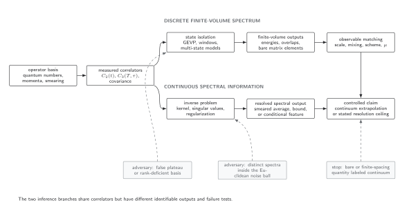
Two inference problems share the same regulated correlators. Discrete energies and overlaps, together with validated connected and disconnected three-point estimators, support bare matrix elements that require matching and continuum control before becoming physical results. Continuous reconstruction identifies only smeared averages, bounds, or conditional features at the demonstrated resolution; without separate matching and continuum analysis it ends at a methodological ceiling. Dashed boxes mark failure tests. The diagram is schematic and not to scale.

Observable-level validation checklist

Before reporting a bare matrix element, verify:

• two-point energies and overlaps are shared consistently with the three-point model;
• both $\tau$ and $T-\tau$ contamination are varied and bounded;
• plateau, summation, and multi-state estimates are compared with full covariance;
• every Wick contraction, flavor coefficient, vacuum term, and sign is enumerated;
• the stochastic estimator is unbiased on an exact small system;
• dilution, control variates, and relaxed solves include their correction terms;
• gauge and stochastic variance are separated by an appropriate nested resampling unit;
• source, sink, insertion, and disconnected-loop data retain configuration pairing; and
• the reported quantity is explicitly bare and finite volume.

Exercises

1. Two-sided contamination. Starting from a two-state spectral sum, derive the terms proportional to $e^{-\Delta_i\tau}$ and $e^{-\Delta_f(T-\tau)}$ in a normalized ratio.

Solution

Keep $(m,n)=(0,0),(0,1),(1,0)$ in $C_3$ and divide out the ground-state overlaps, exponentials, and declared kinematic factors. The additive source-side term is

$$\frac{Z_i^{(1)*}}{Z_i^{(0)*}}J_{01}e^{-\Delta_i\tau},$$

where the complex conjugation follows directly from the source overlap in the spectral sum. The sink-side term is

$$\frac{Z_f^{(1)}}{Z_f^{(0)}}J_{10}e^{-\Delta_f(T-\tau)}.$$

If the ratio is written relative to $J_{00}$ rather than as an additive expansion around it, divide both coefficients by $J_{00}$. Both terms remain unless the corresponding transition matrix element or overlap vanishes by symmetry.

2. Unbiased stochastic trace. Prove $\mathbb E[\eta^\dagger A\eta]=\operatorname{Tr}A$ from the noise second moment.

Solution

$$\mathbb E[\eta^\dagger A\eta] =\sum_{ij}A_{ij}\mathbb E[\eta_i^*\eta_j] =\sum_{ij}A_{ij}\delta_{ij} =\operatorname{Tr}A.$$

The proof fails for an inexact solve because the effective matrix applied to $\eta$ is then not exactly $A$.

What you can now do

You should now be able to decompose a three-point function into ground, excited, connected, disconnected, and vacuum pieces, and to validate a stochastic all-to-all estimator without confusing noise reduction with unbiasedness. Continue with Nonperturbative Renormalization, Mixing, and Step Scaling when the goal is a renormalized matrix element, or with Spectral Reconstruction and Ill-Posed Euclidean Inverse Problems when the target is continuous spectral information.

References

• Dong, Shao-Jing, and Keh-Fei Liu. “Stochastic Estimation with $Z_2$ Noise.” Physics Letters B 328, nos. 1–2 (1994): 130–136. doi:10.1016/0370-2693(94)90440-5.
• Foley, Justin, K. Jimmy Juge, Alan Ó Cais, Mike Peardon, Sinéad M. Ryan, and Jon-Ivar Skullerud. “Practical All-to-All Propagators for Lattice QCD.” Computer Physics Communications 172, no. 3 (2005): 145–162. doi:10.1016/j.cpc.2005.06.008.
• OpenAI Codex for QFT.org. “Lattice Observables and Continuum Inference Benchmark.” JavaScript source, validated 25 August 2026. SHA-256 d76924d8c724cb7c9307fb38265336495fa3ff1a98103b3fa4fa734262647c2a. Reproducibility record.
• Maiani, Luciano, Guido Martinelli, Mario L. Paciello, and B. Taglienti. “Scalar Densities and Baryon Mass Differences in Lattice QCD with Wilson Fermions.” Nuclear Physics B 293 (1987): 420–444. doi:10.1016/0550-3213(87)90078-2.