Scalar Lattice Actions and Difference Operators

A controlled scalar discretization replaces derivatives by local difference operators whose adjoints match the declared boundary conditions. For the standard nearest-neighbor action, variation gives the lattice Klein–Gordon equation, the quadratic form is nonnegative for $m_0^2\ge0$ , and the lattice Laplacian differs from the continuum one first at $O(a^2)$ . These properties must be derived together: a stencil that has the right Taylor series can still fail boundary consistency, Hermiticity, reflection positivity, or locality.

Required background. Lattice Geometry, Boundaries, and Anisotropy fixes the sites, cells, boundaries, and spacings. The Action Principle and Field Equations supplies the variational logic used below.

Helpful background. Field Variations and Boundary Terms gives the continuum summation-by-parts analogue and the role of operator domains.

Difference operators and their adjoints

On an orthogonal lattice, define forward and backward differences by

(\nabla_\mu^+f)_x =\frac{f_{x+a_\mu\hat\mu}-f_x}{a_\mu}, \qquad (\nabla_\mu^-f)_x =\frac{f_x-f_{x-a_\mu\hat\mu}}{a_\mu}.

Their average is the symmetric difference

(\nabla_\mu^{\mathrm s}f)_x =\frac{f_{x+a_\mu\hat\mu}-f_{x-a_\mu\hat\mu}}{2a_\mu},

and the nearest-neighbor Laplacian is

(\Delta_af)_x =\sum_\mu(\nabla_\mu^-\nabla_\mu^+f)_x =\sum_\mu \frac{f_{x+a_\mu\hat\mu}-2f_x+f_{x-a_\mu\hat\mu}}{a_\mu^2}.

With the lattice inner product

(f,g)_a=\left(\prod_\mu a_\mu\right)\sum_x f_x^*g_x,

periodic or consistently twisted boundaries give

(f,\nabla_\mu^+g)_a =-(\nabla_\mu^-f,g)_a.

Thus $(\nabla_\mu^+)^\dagger=-\nabla_\mu^-$ and $-\Delta_a$ is self-adjoint and nonnegative. On an open lattice, the equality acquires the boundary term derived on the geometry page. The adjoint is therefore a statement about the operator together with its domain; it cannot be inferred from the interior stencil alone.

Regulator and conventions. We use a real scalar on a flat Euclidean orthogonal lattice, the weight $e^{-S_a}$ , and the site-wide conventions. The field normalization is chosen so that $[\phi]=(d-2)/2$ in mass units, $[a_\mu]=-1$ , and the lattice action is dimensionless. Boundary conditions are part of every adjoint relation.

For a smooth function sampled on the lattice, Taylor expansion gives

\begin{aligned} \nabla_\mu^+f &=\partial_\mu f+\frac{a_\mu}{2}\partial_\mu^2f +\frac{a_\mu^2}{6}\partial_\mu^3f+O(a_\mu^3),\\ \nabla_\mu^{\mathrm s}f &=\partial_\mu f+\frac{a_\mu^2}{6}\partial_\mu^3f +O(a_\mu^4),\\ \Delta_af &=\partial^2f+\sum_\mu\frac{a_\mu^2}{12}\partial_\mu^4f +O(a^4\partial^6f). \end{aligned}

The forward derivative has an $O(a)$ pointwise error, but the standard kinetic action built from $(\nabla^+\phi)^2$ is symmetric after summation by parts and has an $O(a^2)$ bulk dispersion error. The order of the pointwise stencil and the order of an observable are related but not interchangeable claims.

Deriving the nearest-neighbor field equation

Let $v_a=\prod_\mu a_\mu$ and take

S_a[\phi] =v_a\sum_x\left[ \frac12\sum_\mu(\nabla_\mu^+\phi_x)^2 +\frac12m_0^2\phi_x^2 +V_{\mathrm{int}}(\phi_x) \right].

Vary $\phi_x\mapsto\phi_x+\varepsilon\eta_x$ . To first order,

\delta S_a =v_a\sum_x\left[ \sum_\mu(\nabla_\mu^+\phi_x)(\nabla_\mu^+\eta_x) +\bigl(m_0^2\phi_x+V_{\mathrm{int}}'(\phi_x)\bigr)\eta_x \right].

Periodic summation by parts moves the difference operator from $\eta$ to $\phi$ :

\delta S_a =v_a\sum_x\eta_x \left[ -\Delta_a\phi_x+m_0^2\phi_x+V_{\mathrm{int}}'(\phi_x) \right].

Because the variations are independent, the lattice Euler–Lagrange equation is

-\Delta_a\phi_x+m_0^2\phi_x+V_{\mathrm{int}}'(\phi_x)=0.

On an open lattice, stationarity additionally requires either fixed boundary variations or a boundary equation that cancels the surface term. This is the first adversarial test of a proposed action: vary it with the actual boundary rule rather than varying an infinite-lattice formula and truncating afterward.

For the free theory, summation by parts also gives

S_a=\frac{v_a}{2}\sum_x \phi_x(-\Delta_a+m_0^2)\phi_x.

The quadratic form satisfies

(\phi,(-\Delta_a+m_0^2)\phi)_a =\sum_\mu\lVert\nabla_\mu^+\phi\rVert_a^2 +m_0^2\lVert\phi\rVert_a^2\ge0

for $m_0^2\ge0$ . It is strictly positive for $m_0^2>0$ . At $m_0=0$ with periodic boundaries, constant fields saturate the bound, exposing the zero mode instead of hiding it.

Momentum symbol and the cutoff expansion

For a plane wave $f_x=e^{ip\cdot x}$ ,

\nabla_\mu^+\longmapsto \frac{e^{ia_\mu p_\mu}-1}{a_\mu}, \qquad -\Delta_a\longmapsto \widehat p^2 =\sum_\mu\frac{4}{a_\mu^2} \sin^2\!\left(\frac{a_\mu p_\mu}{2}\right).

This supplies an independent route to positivity: $\widehat p^2\ge0$ throughout the Brillouin zone. Expanding at fixed physical momentum gives

\widehat p^2 =p^2-\sum_\mu\frac{a_\mu^2p_\mu^4}{12} +O(a^4p^6).

The correction is not rotationally invariant: $\sum_\mu p_\mu^4$ distinguishes lattice directions with the same $p^2$ . This is precisely why comparing on-axis and diagonal momenta is a useful symmetry-restoration test.

The same expansion can be represented by a continuum effective action,

S_{\mathrm{eff}} =\int\mathrm d^dx\left[ \frac12(\partial\phi)^2 +\frac12m_0^2\phi^2 -\sum_\mu\frac{a_\mu^2}{24} (\partial_\mu^2\phi)^2 +O(a^4) \right],

up to integration by parts and field redefinitions. This tree-level expression diagnoses the leading free artifact. The full Symanzik expansion of an interacting theory must include every higher-dimension operator allowed by lattice symmetries and its matched coefficient Symanzik 1983, Part I, §§2–3.

Alternative stencils and what they can spoil

One may cancel the $O(a^2)$ Laplacian error in one dimension with a five-point stencil,

(\Delta_a^{(4)}f)_n =\frac{-f_{n+2}+16f_{n+1}-30f_n+16f_{n-1}-f_{n-2}}{12a^2},

whose symbol agrees with $-p^2$ through $O(a^4p^6)$ . This is a valid local improvement in the sense that its range remains finite in lattice units. It also introduces next-nearest-neighbor couplings. If applied in Euclidean time, those couplings can complicate or violate a simple positive transfer-matrix construction. A smaller Taylor error therefore does not imply a uniformly better regulator.

Similarly, the symmetric first derivative has extra zeros at the Brillouin-zone edge. For a scalar kinetic term one normally uses the Laplacian rather than squaring $\nabla^{\mathrm s}$ ; the latter would produce

\left|\frac{\sin(ap)}{a}\right|^2,

which vanishes at both $p=0$ and $p=\pi/a$ . The near-miss anticipates fermion doubling: a locally accurate derivative can have global Brillouin-zone structure that adds unwanted low-energy modes.

Failure modes and independent checks

Taylor accuracy without an adjoint. A stencil can approximate $\partial_\mu$ in the interior while failing the declared boundary inner product. Check summation by parts on the finite lattice.

Positivity checked only near $p=0$ . The continuum expansion says nothing about eigenvalues near the Brillouin-zone boundary. Plot or bound the exact symbol over the full zone.

Interaction dimensions lost in lattice units. Setting $a=1$ is harmless only after every dimensionless coupling has been defined. In $d$ dimensions, a $\lambda\phi^4/4!$ term has lattice coefficient $a^d\lambda$ multiplying fields with their declared normalization.

Improvement treated as continuum proof. Canceling a tree-level $a^2$ term neither tunes all relevant operators nor establishes the interacting continuum limit. Matching and extrapolation belong to Lattice Perturbation Theory, Symanzik Analysis, and Improvement.

Boundary terms inferred from the bulk. An open-boundary action needs its own variational derivation. Periodic index shifting cannot be reused at the edge.

The map below places the stencil calculation between the declared geometry and the observable dispersion test. It makes clear why a locally accurate difference operator cannot be assessed without its boundary mode set, anisotropy calibration, and continuum restoration checks.

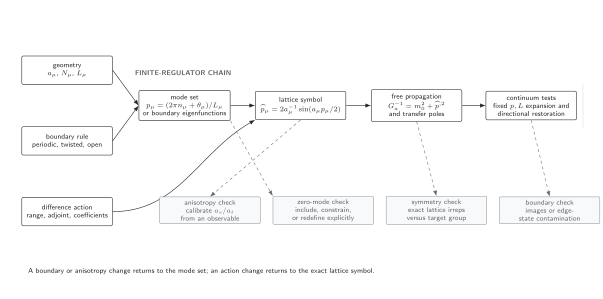
A declared lattice geometry and boundary condition determine discrete modes; finite differences determine trigonometric lattice momenta and free dispersion; separate branches mark anisotropy calibration, zero-mode treatment, exact lattice symmetries, and continuum restoration tests. — Geometry and action data jointly determine finite-regulator propagation. Periodic, twisted, open, and anisotropic choices cannot share one momentum or dispersion formula without translation. The continuum expansion is a tested limit, not an identification at finite spacing. The diagram is schematic and not to scale.

Observable-level validation checklist

Before using a scalar action, verify:

locality by listing the largest stencil separation in physical and lattice units;
adjointness through finite-lattice summation by parts with the actual boundaries;
the lattice equation by direct variation of at least one interior and one boundary variable;
dimensions before setting $a=1$ ;
positivity or the intended instability from the complete eigenvalue spectrum;
the exact momentum symbol over the entire Brillouin zone;
the leading small-momentum artifact and its directional dependence; and
compatibility of any temporal improvement with reflection positivity and transfer interpretation.

Exercises

1. Direct variation. Vary the one-dimensional periodic free action

S=\frac a2\sum_n\left[ \left(\frac{\phi_{n+1}-\phi_n}{a}\right)^2+m_0^2\phi_n^2 \right]

with respect to $\phi_j$ and recover the lattice field equation.

Solution

$\phi_j$ occurs in the links $(j-1,j)$ and $(j,j+1)$ . Differentiation gives

\frac{\partial S}{\partial\phi_j} =a\left[ \frac{2\phi_j-\phi_{j+1}-\phi_{j-1}}{a^2} +m_0^2\phi_j \right] =a(-\Delta_a+m_0^2)\phi_j.

Setting this to zero reproduces the equation derived by summation by parts.

2. The squared symmetric derivative. Show that an action built from $(\nabla^{\mathrm s}\phi)^2$ has an additional zero at $p=\pi/a$ . Why is the continuum Taylor expansion insufficient to reveal it?

Solution

$\nabla^{\mathrm s}$ has symbol $i\sin(ap)/a$ , so the quadratic kernel contains $\sin^2(ap)/a^2$ , which vanishes at $ap=0$ and $ap=\pi$ . A Taylor expansion about $p=0$ has a finite radius that does not encode the global zero at the opposite edge of the Brillouin zone. The exact periodic symbol is the required check.

What you can now do

You should now be able to derive a lattice Euler–Lagrange equation including boundary terms and to test locality, adjointness, positivity, dimensions, and cutoff order independently. Continue with Lattice Momentum, Propagators, and Cutoff Dispersion to invert the quadratic kernel and interpret its Brillouin-zone poles and zero modes.

References

Symanzik, Kurt. “Continuum Limit and Improved Action in Lattice Theories. I. Principles and $\phi^4$ Theory.” Nuclear Physics B 226, no. 1 (1983): 187–204. doi:10.1016/0550-3213(83)90468-6.

References

Section titled “References”- Symanzik, Kurt. “Continuum Limit and Improved Action in Lattice Theories. I. Principles and Theory.” Nuclear Physics B 226, no. 1 (1983): 187–204. doi:10.1016/0550-3213(83)90468-6.
Further reading
Section titled “Further reading”- Montvay, István, and Gernot Münster. Quantum Fields on a Lattice. Cambridge University Press, 1994, §§1.2–1.4. doi:10.1017/CBO9780511470783.
- Rothe, Heinz J. Lattice Gauge Theories: An Introduction. 4th ed. World Scientific, 2012, ch. 2. doi:10.1142/8229.
- Smit, Jan. Introduction to Quantum Fields on a Lattice. Cambridge University Press, 2002, chs. 2–3. doi:10.1017/CBO9780511583971.
Original QFT.org content:CC BY 4.0, unless an item supplies different terms. Third-party material retains its own terms.