Light-Front Coordinates and Quantization

Quantization on the null plane $x^+=0$ turns $x^+$ into the evolution parameter, $P^-$ into the Hamiltonian, and the invariant mass $M^2=2P^+P^- - \mathbf P_\perp^2$ into the natural spectral operator. Seven Poincaré generators preserve the plane and are kinematical; the remaining three contain the interaction. The simplification is real, but the surface is characteristic: canonical momenta become constraints, $\partial_-$ has a kernel, and the $p^+=0$ sector requires separate boundary data. A regulated light-front theory is therefore defined by its null-surface brackets and its longitudinal, transverse, zero-mode, gauge, and Hilbert-space prescriptions.

Required background. Regulated Hamiltonian Field Theory supplies the domain, constraint, and regulator data that make a Hamiltonian spectral problem meaningful. Lorentz Field Representations and Poincaré Particle Representations supplies the Poincaré algebra and the distinction between invariant and frame-dependent labels.

Helpful background. Vacua, States, and Representations clarifies why a Fock vacuum, a physical vacuum, and a representation of the observable algebra need not be identical notions.

Null coordinates and characteristic evolution

Convention and regulator card. This page inherits the site metric $(+---)$ and Fourier phase $e^{-ip\cdot x}$. In $3+1$ dimensions it uses $x^\pm=(x^0\pm x^3)/\sqrt2$ and the same definition for $p^\pm$. The null plane is $x^+=0$. When a finite longitudinal box is used, $x^-$ has period $L_-$; the $p^+=0$ mode is retained as a separate constrained variable, not included in $\partial_-^{-1}$. Transverse space is initially continuous; every later transverse or basis cutoff must be stated independently.

The coordinate change has unit absolute Jacobian in the $(0,3)$ plane and gives

$$\begin{aligned} \mathrm ds^2 &=2\,\mathrm dx^+\mathrm dx^- -\mathrm d\mathbf x_\perp^2,\\ p\mathbin{\cdot}x &=p^-x^+ +p^+x^- -\mathbf p_\perp\mathbin{\cdot}\mathbf x_\perp,\\ p^2&=2p^+p^- -\mathbf p_\perp^2,\\ \mathrm d^4x&=\mathrm dx^+\,\mathrm dx^-\,\mathrm d^2x_\perp . \end{aligned}$$

Thus $p^-$, not $p^+$, is conjugate to light-front time. A free on-shell particle with mass $m$ obeys

$$p^- = \frac{m^2+\mathbf p_\perp^2}{2p^+}.$$

For a future-directed massive momentum, $p^+>0$. This positivity explains why a finite-$P^+$ state admits momentum fractions $x_i=p_i^+/P^+$ with $x_i>0$ and $\sum_i x_i=1$. It does not remove distributions, constrained fields, or global degrees of freedom supported at $p^+=0$. The coordinate and mass-shell translation above differs by factors of $\sqrt2$ and $2$ from the common convention $x^\pm=x^0\pm x^3$; the invariant round-trip check is always $p^2=m^2$. The front-form construction and both normalizations are compared in Heinzl 2000, §§ 2.2–2.3, preprint pp. 10–18, PDF.

A null plane is not a spacelike Cauchy surface. Its normal is tangent to the surface, so the field equation is first order in $\partial_+$ after the longitudinal derivative is isolated. Data for the nonzero longitudinal modes on one null plane can determine their evolution, but uniqueness also depends on boundary or second-characteristic data and on how the zero mode is fixed. That is the geometric reason constraints appear before any interaction has been added.

Kinematical and dynamical generators

The generators that map $x^+=0$ into itself can be represented without the interaction. In $3+1$ dimensions they are

$$P^+,\quad P^1,\quad P^2,\quad M^{12},\quad M^{+-},\quad M^{+1},\quad M^{+2}.$$

The evolution generator $P^-$ and the two rotations $M^{-1},M^{-2}$ that tilt the front are dynamical. This seven-plus-three division is Dirac’s front form Dirac 1949, pp. 392–399. It has two practical consequences.

First, longitudinal and transverse boosts act simply on the internal variables

$$x_i=\frac{p_i^+}{P^+}, \qquad \mathbf k_{\perp i}=\mathbf p_{\perp i}-x_i\mathbf P_\perp, \qquad \sum_i\mathbf k_{\perp i}=0.$$

Second, ordinary spatial rotations are not all manifest. A truncated Hamiltonian may have exact $J^3$ while splitting states that should form one rotation multiplet. Restoring those degeneracies and the Poincaré commutators is a dynamical validation problem, not a change of coordinates. The generator classification and separation of center-of-momentum variables are developed in Brodsky, Pauli, and Pinsky 1998, §§ 2E–3A, arXiv PDF pp. 22–39.

A free scalar already has a canonical constraint

For the inherited real-scalar normalization,

$$\mathcal L =\partial_+\phi\,\partial_-\phi -\frac12(\boldsymbol\nabla_\perp\phi)^2 -\frac12m^2\phi^2,$$

the momentum conjugate to $\partial_+\phi$ is $\pi=\partial_-\phi$. Hence

$$\chi(x)\equiv\pi(x)-\partial_-\phi(x)\simeq0$$

is a primary constraint rather than a formula for an independent velocity. After reducing the nonzero-mode phase space, the equal-$x^+$ field bracket is

$$[\phi(x),\phi(y)]_{x^+=y^+} =-\frac{i}{4}\,\operatorname{sgn}(x^- -y^-) \delta^{(2)}(\mathbf x_\perp-\mathbf y_\perp),$$

and differentiation gives

$$[\phi(x),\partial_-\phi(y)]_{x^+=y^+} =\frac{i}{2}\delta(x^- -y^-) \delta^{(2)}(\mathbf x_\perp-\mathbf y_\perp).$$

The factor $1/2$ is the signature of reduced characteristic data. On a periodic interval the displayed sign kernel must be replaced by the inverse of $\partial_-$ on zero-average functions. Because $\partial_-$ annihilates a constant, no inverse exists on the full field space. The derivation from both the action principle and phase-space reduction is given in Heinzl 2000, §§ 3.2–3.3, preprint pp. 22–29, PDF.

The Klein–Gordon equation becomes

$$2\partial_+\partial_-\phi -\boldsymbol\nabla_\perp^2\phi+m^2\phi=0.$$

For $p^+\ne0$, it determines $\partial_+\phi$ after applying $\partial_-^{-1}$. At $p^+=0$ that step fails; integrating the equation over $x^-$ instead supplies a constraint. The next page treats that sector rather than hiding it inside the inverse derivative.

Exact regulated scalar benchmark

Compactify $x^-$ with period $L_-$ and keep positive nonzero momenta

$$p_n^+=\frac{2\pi n}{L_-},\qquad n=1,2,\ldots .$$

For a free massive scalar in $1+1$ dimensions, define the one-particle state $|n\rangle=a_n^\dagger|0\rangle$. The regulated generators act as

$$P^+|n\rangle=p_n^+|n\rangle, \qquad P^-|n\rangle=\frac{m^2}{2p_n^+}|n\rangle .$$

Consequently

$$M_n^2|n\rangle =2P^+P^-|n\rangle =m^2|n\rangle$$

for every represented nonzero mode. This is an exact finite-regulator dispersion check: a missing factor of two or an interchange of $P^+$ and $P^-$ fails immediately. It is not a test of interacting counterterms, the zero-mode constraint, or the infinite-volume limit.

For a many-body eigenstate, translation invariance fixes $P^+$ and $\mathbf P_\perp$, while dynamics resides in

$$\mathcal M^2 =2P^+P^- -\mathbf P_\perp^2, \qquad \mathcal M^2|\Psi(P)\rangle=M^2|\Psi(P)\rangle .$$

This invariant-mass equation is the precise Hamiltonian handoff to the light-front Fock-space treatment.

The regulator is part of the formulation

A finite calculation must declare, separately:

• the longitudinal boundary condition, $L_-$, harmonic resolution or small-$x$ cutoff, and the $p^+=0$ prescription;
• the transverse momentum, lattice, or basis cutoff and any basis scale;
• the allowed Fock sectors and particle number;
• the gauge choice, residual gauge condition, pole prescription, and regulator fields where applicable; and
• the counterterm basis, renormalization conditions, observables, and order of limits.

At finite regulator, the exact statements are only those of the declared finite Hamiltonian and its reduced physical space. The shared map below locates this page at the coordinate and longitudinal-regulator entrance: the other branches show why those definitions must remain visible when basis, sector, and gauge regulators are added. Its full structured equivalent is the light-front regulator table.

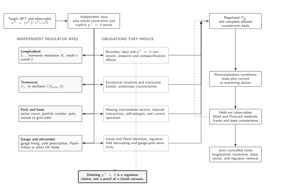
The coordinate convention and longitudinal boundary condition begin, but do not complete, a regulated light-front formulation. The schematic map shows how four independent cutoff axes create distinct obligations before matching, held-out observable tests, and joint limits can support a continuum claim; it is not to scale.

A reproducible free-scalar scan can test the kinematic relations above, but it cannot validate an interacting renormalization claim.

Adversarial failure: positivity used as deletion

Suppose an argument begins with $p^+>0$ for every massive on-shell particle, expands the field only in $p^+>0$ oscillators, and concludes that the vacuum and all constraints are trivial. The first statement is correct in its domain. The conclusion is not: the mode $p^+=0$ is outside the division by $p^+$, lies in the kernel of $\partial_-$, and can carry boundary, gauge, topological, or symmetry-breaking data. Deleting it changes the regulated theory. A valid calculation instead derives its constraint, states a boundary condition, and tests observables against changes of that prescription.

Observable-level validation

Before accepting a light-front quantization, verify all of the following:

• Kinematics: $p\cdot x$, $p^2$, the Fourier phase, and the free dispersion relation survive a round trip to equal-time components.
• Canonical data: the reduced bracket reproduces the field equation and names the kernel of every inverse longitudinal derivative.
• Generators: $M^2$ is independent of the external $P^+$ and $\mathbf P_\perp$ within tolerance, and regulated Poincaré commutator residuals are reported.
• Constraints: zero modes, nondynamical spinor components, Gauss-law data, and residual gauge conditions are either solved or explicitly retained.
• Limits: longitudinal, transverse, basis, Fock-sector, volume, and regulator-field limits are varied independently.
• Observables: at least one held-out mass, current matrix element, Ward identity, or scattering quantity is compared with an independent formulation or exact benchmark.

You should now be able to (1) translate vectors, measures, mass shells, and generators between equal-time and the stated $\sqrt2$ light-front convention, checking $p^2$ and the free scalar mass, and (2) identify the independent scalar data and explain precisely why the zero mode is not fixed by the nonzero-mode bracket. Constrained spinors, gauge fields, and vacuum claims continue in Light-Front Constraints, Zero Modes, and Vacuum Structure; generic equal-time Hamiltonian foundations remain with Hamiltonian Lattice Field Theory, and perturbative scattering observables remain with Perturbative QFT and Scattering.

Exercises

Translate the mass shell

A source uses $X^\pm=X^0\pm X^3$ and writes $p^-_{\mathrm s}=(m^2+\mathbf p_\perp^2)/p^+_{\mathrm s}$. Translate its coordinates and momenta to this page’s convention and recover the displayed factor $1/2$.

Solution

Here $x^\pm=X^\pm/\sqrt2$ and $p^\pm=p^\pm_{\mathrm s}/\sqrt2$. Therefore $p^-=(p^-_{\mathrm s}/\sqrt2) =(m^2+\mathbf p_\perp^2)/(\sqrt2 p^+_{\mathrm s}) =(m^2+\mathbf p_\perp^2)/(2p^+)$. Both conventions give $p^2=2p^+p^- -\mathbf p_\perp^2=m^2$.

Locate the missing canonical datum

On a periodic interval, show that $\partial_- g=f$ has a periodic solution only if $\int_0^{L_-}f\,\mathrm dx^-=0$, and identify the remaining ambiguity.

Solution

Integrating the equation gives $g(L_-)-g(0)=\int_0^{L_-}f\,\mathrm dx^-$. Periodicity makes the left side zero, so the zero-average condition is necessary. It is sufficient after expanding $f=\sum_{n\ne0}f_ne^{2\pi inx^-/L_-}$ and setting $g_n=L_-f_n/(2\pi in)$. The coefficient $g_0$, an arbitrary constant, is not fixed. That undetermined mode is exactly why $\partial_-^{-1}$ must be restricted to the nonzero-mode subspace.

References

• Brodsky, Stanley J., Hans-Christian Pauli, and Stephen S. Pinsky. 1998. “Quantum Chromodynamics and Other Field Theories on the Light Cone.” Physics Reports 301: 299–486. DOI. Open PDF.
• Dirac, P. A. M. 1949. “Forms of Relativistic Dynamics.” Reviews of Modern Physics 21: 392–399. DOI.
• Heinzl, Thomas. 2001. “Light-Cone Quantization: Foundations and Applications.” In Methods of Quantization, Lecture Notes in Physics 572, 55–142. DOI. Open PDF.
• Hiller, John R. 2016. “Nonperturbative Light-Front Hamiltonian Methods.” Progress in Particle and Nuclear Physics 90: 75–124. DOI. Open PDF.