What Counts as a Quantum Simulation of QFT?

A computation counts as a simulation of a target QFT only when it specifies and validates the full map from a renormalized continuum question to a regulated, encoded, prepared, evolved, and measured quantum system. Implementing a finite Hamiltonian is necessary but not sufficient: the observable, physical sector, scale hierarchy, approximation errors, limiting procedure, and matched validation must also be explicit.

Required background. Regulated Hamiltonian field theory supplies the finite Hamiltonian, domain, stability, and continuum-target contract.

Helpful background. Entanglement structure and tensor-network ansätze supplies an independent finite-Hilbert-space representation and classical comparison route.

The object being simulated

Convention and regulator card. Fix a target observable $O_{\rm R}(\mathcal P)$ at renormalized physical parameters $\mathcal P$. A regulator point is $R=(a,L,d_{\rm loc},\mathcal B)$, where $a$ is the spatial spacing, $L$ the physical volume, $d_{\rm loc}$ a local Hilbert dimension or field cutoff, and $\mathcal B$ the boundary condition and sector data. All norms below are finite-dimensional at fixed $R$. Continuum, thermodynamic, infinite-time, and local-dimension limits are distinct and are never silently interchanged.

Quantum simulation is one of several regulated routes to the same continuum target. In the shared formulation map, inspect the last route and its convergence arrow: its finite encoded observable reaches the common claim only after local-Hilbert, volume, time-window, and lattice regulators have been controlled.

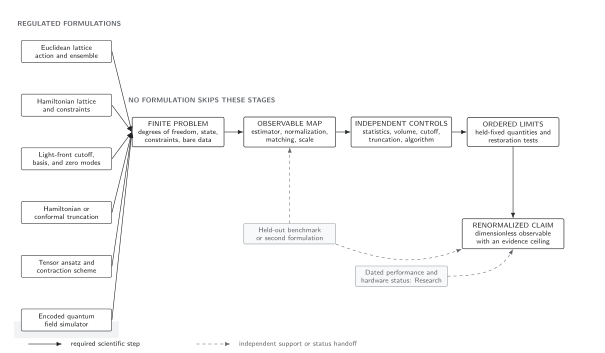
Quantum simulation is a formulation route, not a shortcut around QFT limits. The shared schematic compares regulated formulations by target theory, observable, limit order, and independent error controls. For the quantum route, a finite encoded computation must still establish local-dimension convergence, finite-volume and time-window control, operator matching, and continuum scaling before joining the common dimensionless observable.

At fixed $R$, a digital simulation contract is the tuple

$$\mathcal C_R=(H_R,O_R,\rho_R,V_R,\widetilde H_R, \widetilde O_R,\widetilde\rho_R,\mathcal A,\mathcal M),$$

where $V_R$ maps the regulated physical subspace into the simulator Hilbert space, $\mathcal A$ is the evolution/preparation algorithm, and $\mathcal M$ defines the measurement estimator. The encoded operators should satisfy, on a declared relevant subspace $\mathcal S_R$,

$$\epsilon_H=\bigl\|P_{\mathcal S} (V_RH_RV_R^\dagger-\widetilde H_R)P_{\mathcal S}\bigr\|, \qquad \epsilon_O=\bigl\|P_{\mathcal S} (V_RO_RV_R^\dagger-\widetilde O_R)P_{\mathcal S}\bigr\|.$$

The restricted subspace matters: an unbounded bosonic Hamiltonian cannot have a uniform finite-dimensional operator-norm approximation on its entire Hilbert space.

Analog and continuous-variable simulators use the same logical contract with an experimentally identified effective generator $H_{\rm eff}$. Calibration must determine the parameter map, unwanted terms $\Delta H=H_{\rm eff}-V_RH_RV_R^\dagger$, state preparation, and observable response over a stated time and energy window. An analogy between interactions is not a Hamiltonian match. This bounded use of analog simulation is consistent with the original universal-simulator criterion that controlled local dynamics reproduce another quantum system Lloyd 1996. Continuous-variable scalar-field constructions likewise specify an explicit mode, gate, state, and measurement map Marshall et al. 2015; realizing and calibrating that map requires platform-specific evidence.

From local errors to an observable claim

Let $U=e^{-iH_Rt}$ and $\widetilde U$ be the implemented encoded evolution. For normalized states and a bounded observable, add and subtract intermediate expectations to obtain

$$\begin{aligned} |\widehat O-O_{\rm cont}| \le{}&\epsilon_{\rm reg}+\epsilon_{\rm enc} +\epsilon_{\rm prep}+\epsilon_{\rm evol}\\ &+\epsilon_{\rm meas}+\epsilon_{\rm noise} +\epsilon_{\rm mit}, \end{aligned}$$

where each term must be defined by an operational comparison or bound. For example, if $\|\widetilde O\|\le M$, the trace-distance contribution of state preparation is

$$\left|\operatorname{Tr}\widetilde O (\widetilde\rho- V_R\rho_RV_R^\dagger)\right| \le M\left\|\widetilde\rho-V_R\rho_RV_R^\dagger\right\|_1.$$

If $\|\widetilde H-V_RH_RV_R^\dagger\|\le\epsilon_H$, Duhamel’s formula gives $\|\widetilde U-V_RUV_R^\dagger\|\le t\epsilon_H$ on the controlled subspace, hence an expectation error no larger than $2Mt\epsilon_H$ before state error. This elementary bound is intentionally conservative; it makes visible why a small Hamiltonian mismatch can still matter at long time.

Encoding-to-observable flow

The figure’s upper path is the scientific computation; the lower checks must be attached before a later stage can inherit credibility. Inspect especially the return arrows from measured observables to exact finite-regulator checks.

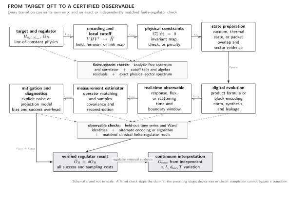
An end-to-end quantum-QFT calculation. Each solid transition carries a state, operator, or observable error; dashed verification paths compare exact limits, physical-sector identities, alternative encodings or algorithms, and matched classical calculations. The map is schematic and platform independent; device execution and changing performance evidence are outside its scale.

Minimum claim–resource–evidence record

This table is a reader-facing stop rule. Every field in a row must refer to the same theory, parameters, observable, accuracy, and confidence level.

Claim tier and target	Regulator, encoding, and constraints	Preparation, algorithm, and observable	Symbolic resources and target error	Matched baseline and verification	Evidence ceiling and handoff
Encoded-system demonstration: reproduce a declared finite-system quantity	Exact finite $a,L,d_{\rm loc}$; explicit qubit, qudit, CV, or analog map; sector projector or “no constraint” stated	Prepared finite-system state; named compiled evolution; bare or encoded observable	Encoded degrees of freedom, depth or analog time, repetitions; norm or observable tolerance	Exact diagonalization or analytic solution; algebra and normalization checks	Demonstration of that encoded system only; report implementation details separately
Regulator calculation: compute a QFT-regulator observable	Tuned finite regulator; encoding convergence; physical-sector leakage bounded	Target state overlap or trace distance; algorithmic error; renormalized finite-regulator estimator	Symbolic dependence on sites, local dimension, time, precision, success probability, and samples	Exact limits, held-out observables, alternate algorithm or encoding, and classical finite-regulator baseline	Finite-regulator QFT statement; no continuum or advantage claim
Continuum-trending result: infer a renormalized observable	Several points on a line of constant physics; $a,L,d_{\rm loc}$ varied independently; constraints restored	Common physical state and observable definition across regulator points	Total uncertainty target allocated across regulator, preparation, evolution, measurement, and statistics	Continuum fit diagnostics, withheld regulator point, cross-formulation or Euclidean comparison	Continuum-trending claim inside demonstrated range; extrapolative reach to Research
Supported advantage: outperform a matched classical route	Same regulator sequence, sector, observable, precision, and confidence for both methods	End-to-end workflows include preparation, postselection, mitigation, and classical preprocessing	Total logical quantum and classical resources with success overhead; assumptions and sensitivity reported	Best available classical baseline, independently reviewed matching, held-out scientific prediction	Necessarily dated comparative assessment in Research; never inferred from qubits, circuit completion, or asymptotic gates alone

The boundary map explains where the last columns live. Inspect the separate continuum and matched-baseline gates: passing one does not imply the other.

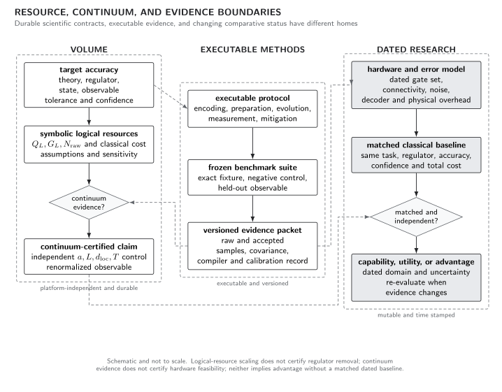
This Volume defines the durable target, regulator, observable, verification, continuum, and symbolic logical-resource contract. Executable protocols require frozen evidence packets. Research records changing physical-hardware assumptions and dated matched-baseline assessments. The schematic contains no current capability or advantage claim.

The scalar-QFT scattering algorithm of Jordan, Lee, and Preskill 2012 is a useful model because it separates discretization, digitization, preparation, scattering evolution, and detection. Its polynomial asymptotic statement holds for its specified problem family and oracle/precision model; it does not certify a device, an arbitrary QFT, or a present-day advantage.

Analytic benchmark: a free periodic chain

For $N=L/a$ periodic sites and $\lambda_0=0$, Fourier modes diagonalize

$$H_0=\frac12\sum_x a\left[\pi_x^2+m_0^2\phi_x^2+ \frac{(\phi_{x+a}-\phi_x)^2}{a^2}\right].$$

With $[\phi_x,\pi_y]=i\delta_{xy}/a$, a unitary site Fourier transform, and $k=2\pi n/L$,

$$\omega_k^2=m_0^2+\frac4{a^2}\sin^2\frac{ka}{2}, \qquad C(t)=\frac1N\sum_k\frac{e^{-i\omega_kt}}{2a\omega_k}.$$

An encoded simulation should reproduce the commutator on its low-energy subspace, the $\omega_k$, the vacuum energy differences, and $C(t)$ before an interaction is enabled. Increasing $d_{\rm loc}$ at fixed $(a,L)$ isolates encoding error; varying the Trotter step at fixed encoding isolates algorithmic error. This triangular test is more informative than agreement at one combined setting.

Adversarial nonexamples

Correct circuit, wrong theory. A circuit exactly implements a spin Hamiltonian whose low-energy terms resemble a gauge theory, but the parameter map and unwanted operators are unmeasured. It is a simulation of the spin Hamiltonian, not yet of the target gauge theory.

Correct Hamiltonian, wrong sector. The encoded Hamiltonian agrees in operator norm, but preparation populates gauge-violating states. A visually plausible correlator does not repair the missing physical-sector condition.

Small finite-system error, unsupported continuum claim. Exact diagonalization validates one $a$, $L$, and $d_{\rm loc}$. A continuum statement still requires a tuned regulator sequence and separate control of finite-volume and local-dimension effects.

Unmatched advantage. A quantum workflow reports only circuit execution while the classical baseline includes continuum fitting, or vice versa. The tasks and accuracies differ, so the comparison has no advantage content.

Observable-level validation checklist

• Freeze the target theory, renormalization condition, external state, observable, physical units, and success tolerance.
• State $a$, $L$, $d_{\rm loc}$, boundary conditions, symmetry sector, and intended limit order.
• Bound or measure encoding error, constraint leakage, preparation error, evolution error, estimator bias, sampling error, and mitigation bias separately.
• Reproduce an analytic or exactly diagonalizable regulator point and at least one held-out observable.
• Repeat one calculation with an independent encoding, algorithm, or classical method and identify shared inputs.
• Report symbolic resources together with success and repetition overhead; send device-specific and comparative status to dated Research evidence.

Exercises

1. Hamiltonian mismatch at finite time

Suppose $\|H-\widetilde H\|\le10^{-3}m$ on the populated subspace, $t=20/m$, and $\|O\|=1$. Use the Duhamel bound to limit the expectation error caused by the Hamiltonian mismatch.

Solution

$\|U-\widetilde U\|\le t\|H-\widetilde H\|=0.02$. The difference between $U^\dagger OU$ and $\widetilde U^\dagger O\widetilde U$ is at most $2\|O\|\|U-\widetilde U\|=0.04$. This is a bound, not an estimate of the typical error.

2. Classify a claim

A simulator reproduces the lowest four energies of an eight-site encoded scalar Hamiltonian at one local cutoff and then measures an interacting correlator. Which claim tier is established?

Solution

At most an encoded-system demonstration. The energy check validates a finite encoded model. A regulator calculation additionally needs encoding convergence, preparation and observable checks, and an error budget; a continuum claim needs a tuned multi-regulator sequence.

Learning outcomes

After working this page, you should be able to:

• Write a complete digital, analog, or continuous-variable simulation contract and attach a quantitative error or falsification test to every map from target QFT to measured observable.
• Given a circuit-fidelity, Hamiltonian-matching, or finite-system result, determine the strongest justified claim tier and list the missing evidence for a regulator, continuum, or advantage statement.

Handoff

Encoding fields and truncating local Hilbert spaces constructs $V_R$, $\widetilde H_R$, and $\widetilde O_R$. Resource and continuum certification converts the completed scientific contract into conditional logical resources. Current platform capability and comparative advantage require a dated Research dossier.

References

• Jordan, Stephen P., Keith S. M. Lee, and John Preskill. “Quantum Algorithms for Quantum Field Theories.” Science 336 (2012): 1130–1133. doi:10.1126/science.1217069.
• Lloyd, Seth. “Universal Quantum Simulators.” Science 273 (1996): 1073–1078. doi:10.1126/science.273.5278.1073.
• Marshall, Kevin, Raphael Pooser, George Siopsis, and Christian Weedbrook. “Quantum Simulation of Quantum Field Theory Using Continuous Variables.” Physical Review A 92 (2015): 063825. doi:10.1103/PhysRevA.92.063825.