Nonperturbative Renormalization, Mixing, and Step Scaling

A bare lattice operator reaches a continuum scheme through a matrix renormalization condition, not a single universal factor. The operator basis must include every mixing partner allowed by exact lattice symmetries, including lower-dimensional terms when present. A nonperturbative condition determines $Z$ in a finite-volume or momentum-subtraction scheme; continuum step scaling moves through a controlled sequence of scales; a final conversion reaches the desired scheme. Infrared contamination, cutoff effects, gauge fixing, chiral breaking, perturbative conversion, and covariance with the bare matrix element remain separate uncertainties.

Required background. Three-Point Functions, Matrix Elements, and Disconnected Contributions supplies the bare operator vector. Nonperturbative Renormalization Schemes and Step Scaling derives the general scheme and RG framework instantiated here.

Helpful background. Operator Mixing and Renormalization Matrices and Renormalization Conditions, Schemes, and Finite Parts explain basis changes and finite scheme conversion.

In the chapter’s observable-chain table, this page supplies the renormalization-and-mixing stage between a bare insertion and the continuum inference.

The lattice operator map

For a closed basis of bare operators $\mathcal O_{0,j}$,

$$\mathcal O_{R,i}^{\mathcal S}(\mu) =Z_{ij}^{\mathcal S}(\mu,a,\mathbf g_0) \mathcal O_{0,j}(a) +\sum_{k:\,d_k<d_i} a^{d_k-d_i}c_{ik}\mathcal Q_{0,k}.$$

The second sum displays possible lower-dimensional mixing. Its coefficients can diverge as powers of $1/a$ and cannot generally be removed by a multiplicative factor. Exact chiral, flavor, gauge, parity, and lattice-spacetime symmetries restrict the basis; hoped-for continuum symmetries do not.

For a vector of bare matrix elements $v_0$, the matched vector is

$$v_R^{\mathcal S}(\mu)=Z^{\mathcal S}(\mu,a)v_0(a)+v_{\mathrm{sub}}(a).$$

Every matrix convention matters: whether operators are row or column vectors, which side $Z$ multiplies, and how projectors are normalized. A round trip through $Z^{-1}$ is the minimal algebraic check.

Renormalization conventions. The page uses the site-wide conventions, a column operator basis, and $\mathcal O_R=Z\mathcal O_0$. The scheme $\mathcal S$, scale $\mu$, gauge condition for off-shell schemes, momentum routing, finite volume, boundary conditions, flavor/chiral basis, and evanescent-operator convention are local. A bare matrix element and $Z$ measured on shared ensembles carry cross-covariance.

Momentum-subtraction conditions

In an RI/MOM-type scheme, compute amputated vertices $\Lambda_j(p)$ for the bare column basis in a fixed gauge. Choose projectors $P_k$ and define

$$M_{kj}(p,a)=P_k\Lambda_j(p,a), \qquad F_{ki}=P_k\Lambda_i^{\mathrm{tree}},$$

with $F$ nonsingular. For $\mathcal O_R=Z\mathcal O_0$, the renormalized vertex carrying operator label $i$ is $\Lambda_{R,i}=\sum_j Z_{ij}\Lambda_j$ times the external-field factors. Therefore the projected condition is

$$\left.MZ^{\mathsf T}D_q\right|_{\mathcal K(p)=\mu}=F, \qquad (D_q)_{\ell i}=\delta_{\ell i}Z_q^{-n_i/2},$$

or, with the sum shown explicitly, $Z_q^{-n_i/2}\sum_jM_{kj}Z_{ij}=F_{ki}$. The transpose is forced by the column-operator convention: the first index of $Z_{ij}$ labels the renormalized operator, whereas the second labels the bare vertex. Ordinary mixing blocks have one external-field content, so $n_i=n$ and $D_q=Z_q^{-n/2}\mathbf1$ within each block; blocks with different external fields are solved separately. Here $Z_q$ renormalizes the external fields and $\mathcal K(p)$ specifies exceptional or nonexceptional momentum kinematics. Solving this equation determines $Z$ only within the declared basis.

The original Rome–Southampton method makes the off-shell renormalization condition computable on the lattice Martinelli et al. 1995, §§2–4. Nonexceptional symmetric kinematics can reduce some infrared channels, but it defines a different scheme and requires its own continuum conversion Sturm et al. 2009.

Because these Green functions are off shell and gauge fixed, a basis closed only among physical gauge-invariant operators may still be incomplete. Operators that vanish by the equations of motion, BRST-exact operators, and gauge-noninvariant operators allowed by the gauge-fixed symmetries can be required to renormalize the off-shell vertices. Their physical on-shell matrix elements may vanish, but omitting them from the intermediate condition can contaminate the extracted physical block of $Z$. State explicitly whether projectors remove these directions or the enlarged basis includes them.

The direct window requirement is

$$\Lambda_{\mathrm{IR}}\ll\mu\ll\frac{\pi}{a}.$$

The lower inequality suppresses condensate, Goldstone-pole, mass, and finite-volume contamination; the upper suppresses lattice artifacts. Hypercubic artifacts also depend on invariants such as $a^2p^{[4]}/p^{[2]}$. A flat-looking $Z(\mu)$ over a narrow interval does not prove both inequalities.

Finite-volume schemes and step scaling

Finite-volume schemes use $L$ itself to define the scale, usually $\mu=c/L$, with boundary conditions and a renormalized coupling specifying the scheme. They avoid a single lattice needing both very large $L$ and very small $a$ at one high scale.

For two scales $\mu_1$ and $\mu_2=s\mu_1$, define the finite-$a$ matrix step

$$\Sigma(\mu_2,\mu_1;a) =Z(\mu_2,a)Z^{-1}(\mu_1,a).$$

At matched renormalized finite-volume conditions, take

$$\sigma(\mu_2,\mu_1) =\lim_{a\to0}\Sigma(\mu_2,\mu_1;a).$$

“Matched” means more than using the same lattice-site count. For each scale step, simulate a sequence of resolutions $L/a$ at the same renormalized coupling, masses, boundary conditions, and physical box size $L$, and pair it with the corresponding sequence for $sL$ or $L/s$ according to the scheme. Extrapolate the resulting matrix ratio in $a/L$ before multiplying it into the running chain. One resolution supplies only $\Sigma$, never the continuum step $\sigma$.

Several steps produce

$$v^{\mathcal S}(\mu_n) =\sigma(\mu_n,\mu_{n-1})\cdots \sigma(\mu_2,\mu_1) v^{\mathcal S}(\mu_1).$$

The multiplication order is fixed by the column convention. A reverse product should recover the starting vector within propagated uncertainty. Step scaling does not remove the need for continuum extrapolation: each $\Sigma$ is a finite-spacing quantity. The Schrödinger-functional program provides a canonical finite-volume realization with recursively connected scales Lüscher et al. 1994.

At a sufficiently high scale, convert to a target continuum scheme $\mathcal T$,

$$v^{\mathcal T}(\mu_n) =C^{\mathcal T\leftarrow\mathcal S}(\mu_n) v^{\mathcal S}(\mu_n).$$

If $C$ is perturbative, truncation error must be estimated independently—for example through order variation, scale variation interpreted within the known series, or comparison of intermediate schemes. Agreement between two schemes after using the same truncated conversion is correlated evidence.

Mixing, chiral symmetry, and gauge constraints

Four-fermion operators illustrate the danger. Several Dirac and color structures can share the same lattice quantum numbers. A regulator that breaks chiral symmetry can allow mixings forbidden in the continuum chiral basis. The $Z$ matrix must be large enough to capture them, and projectors must be linearly independent in the chosen kinematics.

Lower-dimensional mixing is more severe. If $\mathcal O_d$ mixes with $\mathcal Q_{d-r}$, the coefficient can scale as $a^{-r}$. Subtracting two large numbers to obtain a finite matrix element magnifies small coefficient errors. A symmetry that forbids the mixing or a nonperturbative subtraction condition is required; a smooth continuum plot after an ad hoc subtraction is not enough.

Gauge-fixed off-shell schemes introduce gauge dependence into $Z^{\mathcal S}$, while a properly converted physical matrix element must be gauge independent. Gauge-parameter variation can diagnose errors but does not replace a complete conversion. Gribov-copy effects and finite-volume gauge fixing must be bounded at the precision claimed.

Covariance through the complete chain

Let

$$\sigma_k=\sigma(\mu_{k+1},\mu_k), \quad k=1,\ldots,n-1, \qquad S=\sigma_{n-1}\sigma_{n-2}\cdots\sigma_1.$$

For a column vector, later scale steps therefore multiply on the left. Define the ordered partial products

$$S_{>k}=\sigma_{n-1}\cdots\sigma_{k+1}, \qquad S_{<k}=\sigma_{k-1}\cdots\sigma_1,$$

with an empty product equal to the identity. If $v_R=SZv_0$, variations satisfy

$$\delta v_R =SZ\,\delta v_0 +S(\delta Z)v_0 +\sum_k S_{>k}(\delta\sigma_k)S_{<k}Zv_0.$$

This Jacobian propagates the joint covariance. When $v_0$ and $Z$ share gauge ensembles, the cross term can be important. Resampling all stages together is preferable when possible; otherwise the cross-covariance must be estimated or conservatively bounded.

The QFT.org 2026 Chapter 2 benchmark, validated snapshot evolves a vector through noncommuting mixing and step matrices, recovers it with the reverse-ordered inverse chain to $1.2\times10^{-16}$ in Euclidean norm, and produces a $0.019987$ shift for the deliberately reversed forward product. These are deterministic algebraic cross-checks, not a determination of any physical $Z$ matrix.

The renormalization-continuum figure on the tuning page places this matrix chain between state isolation and continuum fitting. Renormalization and scale setting are distinct: $\mu$ labels a scheme scale, while $a$ converts lattice units.

Adversarial failure cases

Diagonal $Z$ assumed from continuum quantum numbers. Finite-$a$ exact symmetries determine the mixing blocks. Test every off-diagonal element allowed by them.

No scale window. If $\mu$ is comparable with both $\Lambda_{\mathrm{IR}}$ and $1/a$, a stable answer can reflect cancellation between unrelated contaminations.

Step scaling performed at one $a/L$. That is a finite-regulator ratio, not the continuum step function.

Matrix order reversed. Noncommuting mixing matrices make this a real numerical error. Apply a known vector and verify forward and inverse round trips.

Conversion uncertainty omitted. A nonperturbative intermediate scheme does not make the final truncated conversion nonperturbative.

Shared-ensemble covariance ignored. Treating $v_0$ and $Z$ as independent can understate or overstate the final error.

The map below places mixing and step scaling within the full observable chain. Follow the path on both sides of the matching stage: the bare matrix element must already be controlled, and scheme conversion still has to feed a correlated continuum extrapolation and a held-out prediction.

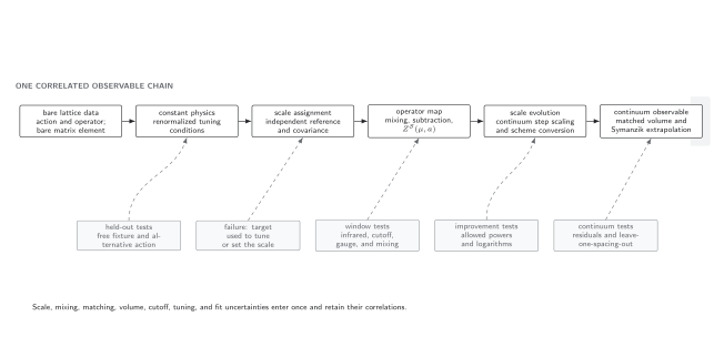
A continuum prediction requires a tuned bare trajectory, a regulator-consistent calculation, and a renormalized observable in a named scheme. When momentum-space lattice perturbation theory is used, its propagators, vertices, and Brillouin zone must be retained unless a controlled matching or subtraction justifies a continuum replacement. Step scaling or scheme conversion is optional when the matching scale is already suitable. The failure exits reject an untuned trajectory, an unjustified continuum propagator inside a lattice loop, a defining input counted as a prediction, and a one-spacing or unsupported extrapolation. Schematic, not to scale.

Observable-level validation checklist

Before reporting $v_R^{\mathcal T}(\mu)$, require:

• a symmetry-complete operator and lower-dimensional subtraction basis;
• nonsingular tree-level projector matrix and declared momentum kinematics;
• gauge, mass, volume, and hypercubic-artifact studies;
• evidence for an infrared–cutoff window or a finite-volume step-scaling alternative;
• continuum extrapolation of every step matrix;
• matrix multiplication and reverse-evolution round trips;
• perturbative conversion order and truncation uncertainty;
• Ward-identity or protected-operator cross-checks where available;
• full covariance among bare matrix elements, $Z$, scale steps, and conversion; and
• agreement of a physical quantity through a second intermediate scheme when precision warrants it.

Exercises

1. Mixing round trip. Given invertible matrices $Z,S_1,S_2$, show that the inverse chain recovering $v_0$ from $v_R=S_2S_1Zv_0$ is $Z^{-1}S_1^{-1}S_2^{-1}$.

Solution

Matrix inverses reverse order:

$$Z^{-1}S_1^{-1}S_2^{-1}v_R =Z^{-1}S_1^{-1}S_2^{-1}S_2S_1Zv_0=v_0.$$

Using $S_2^{-1}S_1^{-1}Z^{-1}$ instead generally fails because the matrices need not commute.

2. Power-divergent sensitivity. If $O_R=O_0-c(a)Q_0/a^2$ and $c$ has relative error $\varepsilon$, estimate the subtraction error.

Solution

The induced error is $\delta O_R\simeq-\varepsilon c(a)Q_0/a^2$. It grows as $a^{-2}$ unless $Q_0$ or $c$ supplies compensating scaling. A fixed relative precision on $c$ is therefore not enough for a finite continuum uncertainty.

What you can now do

You should now be able to construct a matrix renormalization condition, diagnose its scale window, evolve it through continuum step-scaling matrices, and propagate the result with the bare observable covariance. Continue with Lattice Perturbation Theory, Symanzik Analysis, and Improvement to compute lattice-side matching coefficients and predict the remaining cutoff powers.

References

• Lüscher, Martin, Rainer Sommer, Peter Weisz, and Ulli Wolff. “A Precise Determination of the Running Coupling in the SU(3) Yang–Mills Theory.” Nuclear Physics B 413, nos. 3–4 (1994): 481–502. doi:10.1016/0550-3213(94)90629-7.
• Martinelli, Guido, Christopher T. Sachrajda, Christopher Pittori, Mario Testa, and Anna Vladikas. “A General Method for Non-Perturbative Renormalization of Lattice Operators.” Nuclear Physics B 445, no. 1 (1995): 81–105. doi:10.1016/0550-3213(95)00126-D.
• OpenAI Codex for QFT.org. “Lattice Observables and Continuum Inference Benchmark.” JavaScript source, validated 25 August 2026. SHA-256 d76924d8c724cb7c9307fb38265336495fa3ff1a98103b3fa4fa734262647c2a. Reproducibility record.
• Sturm, Christian, Yao Aoki, Norman H. Christ, Taku Izubuchi, Christopher T. Sachrajda, and Amarjit Soni. “Renormalization of Quark Bilinear Operators in a Momentum-Subtraction Scheme with a Nonexceptional Subtraction Point.” Physical Review D 80, no. 1 (2009): 014501. doi:10.1103/PhysRevD.80.014501.