DLCQ and Basis Light-Front Quantization

Discrete light-cone quantization (DLCQ) makes longitudinal momentum fractions rational at fixed harmonic resolution $K$, while basis light-front quantization (BLFQ) also expands transverse motion in a finite orthonormal basis. The invariant-mass equation then becomes a sparse matrix eigenproblem inside fixed momentum, charge, and kinematical-symmetry sectors. Finite matrix dimension is not the continuum limit: $K$, longitudinal volume, transverse resolution, basis scale, Fock sectors, zero-mode prescription, and counterterms remain independent parts of the calculation.

Required background. Light-Front Constraints, Zero Modes, and Vacuum Structure supplies the boundary data that compactification cannot choose automatically. Light-Front Fock Space, Wavefunctions, and Bound-State Equations supplies the coupled invariant-mass equations and state normalization being discretized.

Helpful background. Normal Forms, Spectra, and Projectors supplies finite-dimensional spectral decomposition, symmetry blocks, and residual checks.

Harmonic resolution makes longitudinal partitions finite

Convention and regulator card. Work first in $1+1$ dimensions with $x^\pm=(x^0\pm x^1)/\sqrt2$, periodic $x^-$ of length $L_-$ for a scalar, and $p_n^+=2\pi n/L_-$. Positive modes have integer $n\ge1$; the $n=0$ mode is retained as a separate constraint. Total momentum is $P^+=2\pi K/L_-$. A transverse BLFQ extension declares $(N_{\max},b)$, every Fock sector, and all ultraviolet regulators in addition to $K$ and $L_-$.

At fixed total $P^+$, longitudinal momentum conservation becomes

$$\sum_{i=1}^N n_i=K, \qquad x_i=\frac{n_i}{K}, \qquad n_i\in\mathbb Z_{>0}.$$

Only finitely many positive-integer partitions exist. If particle number can change but every constituent carries at least one unit, then $N\le K$. This is why DLCQ makes a $1+1$-dimensional Fock basis finite once species and internal quantum numbers are bounded. Identical-particle symmetrization identifies permutations; distinguishable particles or ordered operator strings do not.

Boundary conditions are physical regulator data. Periodic bosons have integer modes and a zero mode. Antiperiodic fermions have half-integer modes, which can simplify the zero-mode bookkeeping but changes the finite-volume theory. Gauge fields and residual gauge transformations require their own consistent boundary treatment. DLCQ’s construction and its relation to the continuum integral equations were introduced in Pauli and Brodsky 1985, pp. 2001–2013 and are reviewed in Brodsky, Pauli, and Pinsky 1998, Chapter 4, arXiv PDF pp. 65–97.

Three quantities that share one equation must not be conflated:

$$K=\frac{P^+L_-}{2\pi}.$$

Increasing $K$ at fixed $L_-$ changes $P^+$; increasing $K$ at fixed $P^+$ changes the box; increasing $P^+$ at fixed fractions is a longitudinal boost only when the regulated formulation preserves that kinematical symmetry. Record which operation is actually performed.

Exact free one- and two-particle benchmarks

For a free scalar of mass $m$ in $1+1$ dimensions, the one-particle state at mode $K$ has

$$P^-_K=\frac{m^2}{2P^+}, \qquad M_1^2=2P^+P^-_K=m^2.$$

Thus every represented one-particle mode must satisfy the dimensionless dispersion residual

$$R_{\mathrm{disp}} =\left|\frac{2P^+P^-_K}{m^2}-1\right|.$$

For two free particles with partition $(n,K-n)$,

$$\begin{aligned} M_{2,n}^2 &=2P^+\left( \frac{m^2}{2p_n^+} +\frac{m^2}{2(P^+-p_n^+)} \right)\\ &=m^2\left(\frac{K}{n}+\frac{K}{K-n}\right) =\frac{m^2K^2}{n(K-n)}. \end{aligned}$$

At even $K$, $n=K/2$ gives the exact threshold $M_2^2=4m^2$. At odd $K$, the closest grid points give

$$M_{2,\min}^2=\frac{4m^2K^2}{K^2-1}>4m^2.$$

The excess is a known momentum-fraction discretization effect, not binding. These formulas check $K$ assignment, mode energies, symmetrization, and matrix units before an interaction is added.

A reproducible free-scalar baseline can use the grid $mL_-=4\pi,6\pi,8\pi$ crossed with $K=4,6,8,12,16$. At fixed box it refines $K$; at fixed $K=8,12$ it varies the box. A correct implementation records the resulting $P^+$ rather than pretending that all three quantities are fixed.

Matrix construction is a reproducible method

A DLCQ calculation can be reproduced from the following contract:

1. Fix the theory. State the regulated $P^-$, fields, masses, couplings, gauge and ordering prescriptions, counterterms, and target observable.
2. Fix the sector. Choose $K$, conserved charge, statistics, boundary conditions, and all kinematical quantum numbers.
3. Enumerate states. Generate every allowed momentum partition and Fock sector exactly once, retaining a separate representation of constrained zero modes.
4. Construct matrix elements. Include kinetic, particle-changing, instantaneous, zero-mode-induced, and counterterm operators with their symmetry and combinatorial factors.
5. Verify structure. Test Hermiticity in the correct inner product, conserved charges, block dimensions, and known free eigenvalues.
6. Solve and diagnose. Compute targeted eigenpairs, residual norms, and wavefunction normalization; do not infer accuracy from eigensolver convergence alone.
7. Repeat regulators. Refit only the declared renormalization inputs at every cutoff point and reserve held-out observables for extrapolation and validation.

The matrix element vanishes unless longitudinal mode numbers satisfy the same integer conservation rule as the continuum delta function. This gives a powerful exact sparsity check. Conversely, a finite matrix that preserves $K$ can still violate a dynamical rotation, omit a zero-mode-induced term, or use the wrong current.

BLFQ supplies a transverse basis, not automatic convergence

In $3+1$ dimensions, longitudinal partitions alone leave continuous transverse momenta. A common BLFQ choice uses two-dimensional harmonic- oscillator functions labeled by radial $n$, azimuthal $m$, and a scale $b$. A many-particle cutoff may be written

$$\sum_i\left(2n_i+|m_i|+1\right)\le N_{\max}.$$

Together with $K$, Fock-sector restrictions, helicity, charges, and total $J^3$, this produces finite symmetry blocks. The original basis-function formulation emphasizes that basis choice affects convenience and convergence, while covariance requires the infinite-basis limit Vary et al. 2010, §§ III–IV, arXiv PDF pp. 5–13.

The oscillator scale $b$ has two possible roles that must be distinguished. If it appears only in a complete basis transformation, exact observables are independent of it and residual $b$ dependence diagnoses truncation. If a trap or confining operator proportional to $b$ is part of the target Hamiltonian, $b$ is physical model data. Treating one role as the other can manufacture a false plateau.

Other smooth bases—splines, orthogonal polynomials, plane waves, wavelets, or problem-adapted functions—replace abrupt momentum grids with different approximation spaces. They still require endpoint behavior, zero-mode data, a complete counterterm basis, and a convergence study. Hiller surveys DLCQ, function expansions, BLFQ, and their distinct regulators in Hiller 2016, §§ 3.1 and 3.4, preprint pp. 15–29, PDF.

Every cutoff needs its own convergence observable

Independent cutoffs in a light-front basis calculation.

Axis	What is omitted	Minimum diagnostic	Required comparison
$K$	Longitudinal fractions between grid points	Fixed-$L_-$ spectrum and wavefunction moments	Several $K$ values at the same box and prescription
$L_-$	Long-range and compactification physics	Mass or matrix element at fixed $K$ values	Several boxes without identifying them with equal-time boxes
$N_{\max}$ or $\Lambda_\perp$	Transverse resolution and ultraviolet states	Energy, radius, and rotational multiplet splitting	Several cutoffs and basis scales
Fock sectors	Virtual intermediate states and induced operators	Sector probabilities and held-out current or scattering datum	Nested sector sets with consistent renormalization
Basis family and scale	Approximation directions poorly represented by one basis	Residual norm and scale sensitivity	A second complete basis or a justified extrapolation model

A diagonal sequence such as $K=N_{\max}=8,10,12$ is useful for cost studies but cannot identify which axis controls the change. At minimum, add fixed-$K$ transverse scans and fixed-$N_{\max}$ longitudinal scans. An interacting calculation must also retune its counterterms according to a fixed protocol; otherwise drift can reflect changing renormalized parameters rather than cutoff error.

The shared map below places $K$ and $L_-$ on the longitudinal branch while keeping transverse or basis and Fock-sector truncations independent. That separation is the graphical counterpart of the table above; the complete constraint and counterterm fields appear in the chapter-spanning regulator table.

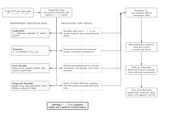
DLCQ resolution, longitudinal compactification, transverse or basis size, and retained sectors are distinct regulator axes. The schematic map requires fixed-axis convergence tests, consistent matching, and held-out observables before their limits are combined; it is not to scale.

Adversarial failure: one smooth diagonal extrapolation

Imagine that three points with $(K,N_{\max},N_F)=(8,8,2),(10,10,3),(12,12,4)$ lie on a smooth curve. The mass appears converged, but longitudinal resolution, transverse resolution, and Fock content changed together. A cancellation among their errors can produce the plateau, and the changing sector count may require different counterterms.

The result supports only stability along that single path. To identify a continuum trend, hold two axes fixed while varying the third, repeat with a second basis or boundary condition, and test a held-out observable. If cost prevents this Cartesian design, the unseparated error is a claim limitation, not zero.

Observable-level validation

• Enumeration: compare basis counts with independent integer-partition code for small $K$ and inspect identical-particle factors.
• Free anchors: reproduce $M_1^2=m^2$ and the two-body formula above to a tolerance set before interacting runs.
• Matrix checks: verify Hermiticity, exact kinematical charges, sparse selection rules, and eigenpair residuals.
• Zero modes: evaluate the integrated constraint rather than silently dropping $n=0$.
• Axis separation: scan $K$, $L_-$, transverse cutoff, basis scale, and Fock sectors independently.
• Symmetry and observables: test frame-independent $M^2$, rotational or Poincaré residuals where available, and at least one matched current or scattering quantity not used in tuning.

You should now be able to (1) construct the complete finite partition basis at fixed $K$ while listing every additional cutoff, and (2) design an extrapolation that separates boundary, zero-mode, longitudinal, transverse, basis, and Fock-sector effects. Light-Front Regulators, Counterterms, and Symmetry Restoration supplies the cutoff-dependent Hamiltonian; generic basis construction and eigensolvers continue in Hamiltonian Truncation and Variational Methods, and dated large-scale performance belongs to Research.

Exercises

Enumerate the $K=6$ scalar sectors

List the unordered two-boson partitions and compute their free invariant masses in units of $m^2$. Identify the threshold state.

Solution

The unordered positive partitions are $(1,5)$, $(2,4)$, and $(3,3)$. The formula $M_{2,n}^2/m^2=K^2/[n(K-n)]$ gives

$$\frac{36}{5},\qquad \frac{36}{8}=\frac92, \qquad \frac{36}{9}=4.$$

The symmetric partition $(3,3)$ reaches the exact free threshold. An ordered basis would also contain the exchanged labels $(5,1)$ and $(4,2)$ before bosonic symmetrization.

Design an identifiable cutoff scan

You can afford nine calculations near $(K,N_{\max})=(12,16)$. Give a design that estimates both one-axis effects and their leading interaction.

Solution

Use a $3\times3$ Cartesian grid, for example $K\in\{8,12,16\}$ and $N_{\max}\in\{12,16,20\}$, with the same $L_-$, Fock sectors, basis scale, zero-mode prescription, renormalization conditions, and held-out observable at every point. Fixed-$N_{\max}$ rows identify the $K$ trend, fixed-$K$ columns identify the transverse trend, and the departure from an additive fit diagnoses an interaction between the two cutoffs. A diagonal set of nine points would spend more computation without providing this identifiability.

References

• Brodsky, Stanley J., Hans-Christian Pauli, and Stephen S. Pinsky. 1998. “Quantum Chromodynamics and Other Field Theories on the Light Cone.” Physics Reports 301: 299–486. DOI. Open PDF.
• Heinzl, Thomas. 2001. “Light-Cone Quantization: Foundations and Applications.” In Methods of Quantization, Lecture Notes in Physics 572, 55–142. DOI. Open PDF.
• Hiller, John R. 2016. “Nonperturbative Light-Front Hamiltonian Methods.” Progress in Particle and Nuclear Physics 90: 75–124. DOI. Open PDF.
• Pauli, Hans-Christian, and Stanley J. Brodsky. 1985. “Discretized Light-Cone Quantization: Solution to a Field Theory in One Space and One Time Dimensions.” Physical Review D 32: 2001–2013. DOI.
• Vary, James P., et al. 2010. “Hamiltonian Light-Front Field Theory in a Basis Function Approach.” Physical Review C 81: 035205. DOI. Open PDF.