Benchmark Theories for Truncation Methods

A benchmark ladder is adequate only when each stage targets a distinct failure mode, compares with an exact or genuinely external reference, and includes an adversarial enlargement of the state or operator basis. The ladder should run from analytic construction tests through weakly coupled and integrable flows to nonintegrable finite-volume QFT, while keeping at least one spectral or matrix-element result blind. Agreement with quantities used to tune counterterms is calibration, not validation.

Required background. Convergence, Extrapolation, and Error Certification supplies the evidence levels, correlated fits, and false-plateau tests used here.

Helpful background. Hamiltonian Continuum Limits and Euclidean Cross-Validation supplies matched cross-formulation observables and independent limit orders.

A benchmark ladder isolates failures before increasing difficulty

Benchmark and blind-prediction contract. For every row, freeze the target Hamiltonian, sector, observable, cutoff sequence, counterterms, reference and its uncertainty, pass tolerance, expected cost, and adversarial enlargement. Mark every fitted datum. Keep held-out values inaccessible until code, matching, fit windows, and uncertainty rules are frozen. A benchmark passes only for the declared theory, observable, range, and tolerance.

The ladder below is ordered by diagnostic purpose rather than by prestige:

Benchmark ladder for Hamiltonian and conformal truncation.
Stage	Reference	Failure exposed	Adversarial enlargement
Free construction	Analytic Fock spectrum, degeneracies, and matrix elements	Units, basis counts, symmetry sectors, normalization	Add modes and complete multiplets
Few-state elimination	Exact two- and three-state diagonalization	Resolvent sign, induced mixing, counterterm insufficiency	Move a state between `P` and `Q`
Anharmonic oscillator	High-precision independent diagonalization or rigorous bounds	Variational bias, strong-coupling scaling, operator moments	Add non-Gaussian states and operators
Integrable deformation	Exact finite-volume or scattering spectrum	CFT normalization, sectors, radius dependence, cutoff tails	Change cutoff rule and retain full multiplets
Weak coupling	Independent perturbation theory	Combinatorics, signs, subtraction, leading running	Include the next perturbative and operator order
Interacting finite-volume QFT	Frozen higher-cutoff or independent formulation	Nonperturbative cutoff and volume extrapolation	Second basis and counterterm basis
Observables and dynamics	Sum rules, Ward identities, exact short-time coefficients	Effective-operator, leakage, phase, and recurrence errors	Cross state and operator cutoffs
Blind cross-method prediction	Sequestered Euclidean, integrable, or independent-basis value	Analysis-choice leakage and shared systematic errors	Unblind only after the full record is signed off

An exact benchmark is valuable only if it probes the same code path as the interacting calculation. Hard-coding a diagonal free Hamiltonian does not test the interaction assembler. Conversely, an interacting reference generated by the same code at a larger cutoff is useful for regression but is not fully independent evidence.

Stage 1: exact construction and omitted-state fixtures

For a free scalar on a circle,

E_{\{N_n\}}=\sum_n\sqrt{m^2+(2\pi n/L)^2}\,N_n

gives every retained energy and degeneracy. Exact momentum and $\mathbb Z_2$ sectors test enumeration. The one-mode ${:}(a+a^\dagger)^4{:}$ matrix tests normalization and interaction combinatorics. These fixtures must pass at several cutoffs, not only in the smallest matrix.

The two-state model

H=\begin{pmatrix}0&g\\g&\Delta\end{pmatrix}

tests the exact Feshbach equation and the dynamical leakage probability. The three-state model on the renormalization page tests induced off-diagonal structure that a single fitted energy cannot determine. Moving the high state from $Q$ into $P$ must leave exact low eigenvalues invariant when the effective Hamiltonian is treated exactly; any discontinuity exposes an implementation or subtraction error.

Stage 2: one interacting degree of freedom

The quartic oscillator

H=\frac{p^2}{2}+\frac{m^2q^2}{2}+\frac{\lambda q^4}{4!}

adds nontrivial convergence without field-theory volume or momentum sectors. It tests Gaussian and non-Gaussian variational families, Fock-energy cutoffs, strong-coupling behavior, moments such as $\langle q^2\rangle$ , and effective operators. The weak-coupling coefficients and high-precision numerical spectrum have a long independent history beginning with Bender and Wu 1969, §§ II–IV.

For $\lambda\to\infty$ , rescaling $q=\lambda^{-1/6}x$ shows that energies scale as $E_n\propto\lambda^{1/3}$ . A method that reproduces small- $\lambda$ perturbation theory but fails this exact exponent has not crossed to the strong coupling regime. A stable energy should be accompanied by at least one moment or transition matrix element.

Stage 3: integrable and weakly coupled field theories

Relevant deformations of two-dimensional CFTs provide exact or independently known finite-volume spectra while exercising conformal Gram matrices, descendants, null states, and cutoff renormalization. The scaling Lee–Yang model was the original TCSA benchmark Yurov and Zamolodchikov 1990, §§ 2–4. The thermal Ising deformation supplies a massive free-Majorana reference after conventions are matched. Because the scaling Lee–Yang theory is nonunitary, it tests TCSA algebra and cutoff treatment but not positive-metric variational bounds.

A weakly coupled finite-volume scalar theory then tests interaction combinatorics and subtraction against independent Rayleigh–Schrödinger perturbation theory. Compare coefficients, not merely final decimal values: vacuum energy, one-particle gap, and a composite-operator matrix element probe different terms. Repeating at two volumes tests whether a purported UV counterterm has accidentally absorbed an infrared effect.

Integrability is not itself a guarantee that the truncation is controlled. The benchmark must include several cutoffs, complete symmetry sectors, and an observable not used to normalize the coupling.

Stage 4: nonintegrable finite-volume φ⁴

Two-dimensional $\phi^4$ theory in a massive free-boson basis supplies a standard nonintegrable test of energy truncation, counterterms, broken and unbroken sectors, and strong coupling. Its finite-volume Hamiltonian and the improvement from renormalization are analyzed in Rychkov and Vitale 2015, §§ 2–4, with phase and duality tests extended in Rychkov and Vitale 2016, §§ 2–5. Next-to-leading effective Hamiltonians provide a sharper test of omitted-state models Elias-Miró, Rychkov, and Vitale 2017, §§ 2–4.

A smaller reproducible baseline uses:

L=2\pi, \qquad m=1, \qquad g=0.5, \qquad H=H_0+\frac{g}{4!}\int_0^L dx\,{:}\phi^4{:}.

It uses zero-momentum even and odd sectors and $E_{\max}=8,10,12,14,16$ . The $g=0$ spectrum is analytic. An interacting $E_{\max}=24$ calculation is frozen as a separate reference for declared comparisons; its values remain hidden until the lower-cutoff matrices, counterterms, fit windows, residual tolerances, and prediction fields are fixed. Vacuum energy, first gap, a $\phi^2$ matrix element, omitted-state correction, operator counterterm, cutoff residual, and eigensolver residual have separate tolerances. Only eligible energies receive variational-bound language.

The same continuum observable can be approached with Euclidean, equal-time Hamiltonian, conformal, light-front, or tensor representations, but their finite regulators are not equal. The map below shows why each route must first remove or quantify its own errors before a shared continuum intercept is meaningful.

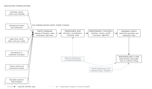
Euclidean lattice, Hamiltonian, light-front, basis-truncation, tensor-network, and quantum-simulation routes each pass from a finite regulator through observable extraction and independent error controls before a continuum claim. — Different finite formulations can support one continuum statement only after their conventions, renormalized observables, regulator axes, and limit orders are matched. Internal numerical convergence is necessary but does not alone establish the target QFT. The diagram is schematic and not to scale.

A cross-formulation comparison is appropriate only after each participating method has passed its own baseline. It must not use a shared reference value during method selection, and common input uncertainties must be retained as correlations rather than counted twice.

As of 9 August 2026, this durable page does not rank current truncation methods or claim a settled precision frontier. Dated reach, cost comparisons, leaderboards, and unresolved disagreements belong to Research: Lattice and Hamiltonian Field Theory, where their source dates and evidence can be updated without changing the method definitions here.

The truncation flow sets the pass condition

Every benchmark must traverse the full map: construction, omitted-state correction, effective observable, independent axes, held-out comparison, and adversarial enlargement. The dashed branch is a failed benchmark even when its fitted energy looks precise.

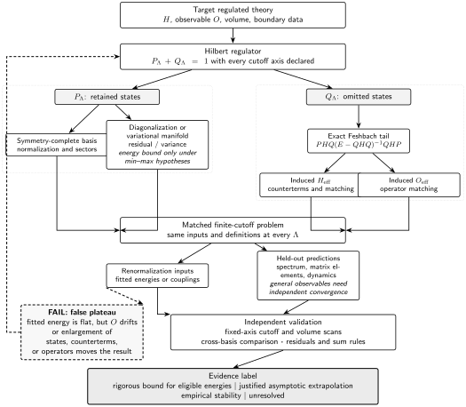
A Hilbert-space cutoff splits retained and omitted states; omitted states induce effective Hamiltonians and observables, while symmetry, variational, residual, cross-basis, and held-out checks determine whether a plateau can support a certified limit — A benchmark passes only after state and operator construction, omitted-state matching, independent cutoff scans, residuals, held-out observables, and cross-basis checks agree. Monotone Ritz energies and general observables carry different evidence, and the schematic false plateau must fail the pass gate.

Minimum truncation certification record

Every benchmark row in this record requires an exact or external reference and an adversarial state- or operator-basis enlargement. Internal agreement alone does not close the row.

Required fields for a truncation result and the test that can falsify each field.
Field	Required declaration	Independent test	Failure signal
Target	Hamiltonian, prior regulator, volume, boundary data, observable	Units and free or exact limit	Changing target across cutoff points
Projectors	`P`_Λ, `Q`_Λ, all cutoff axes, limit order	State counts and nestedness	Unidentified omitted states
Basis and sectors	Normalization, Gram matrix, null removal, exact charges	Hermiticity and selection rules	Duplicates or broken constraints
Induced Hamiltonian	Derived operator basis and approximation order	Omitted-state toy model or perturbative coefficient	Drift incompatible with the declared tail
Counterterms	Inputs, running coefficients, and no-double-counting rule	Refit protocol at every cutoff	A fitted datum presented as a prediction
Variational status	Manifold, optimizer, symmetry, bound hypotheses	Residual, variance, and ansatz enlargement	Energy plateau with a large residual
Effective observables	Projected and induced operator terms	Sum rule or matched matrix element	Spectrum stable while the observable drifts
Cutoff sequence	Independent basis, volume, counterterm, time, and state scans	Fixed-axis and cross-term fits	Only one diagonal sequence
Extrapolation	Asymptotic form, fit window, covariance, alternatives	Window and model stability	Exponent chosen from the desired answer
Held-out tests	Unused spectrum, matrix element, dynamics, and second basis	Blind comparison after choices freeze	All tests participated in tuning
Adversarial enlargement	Larger state and operator bases	Repeat the full match and prediction	Former plateau moves beyond its error
Claim	Bound, asymptotic evidence, empirical stability, or unresolved	Error and cost reproduced independently	Precision exceeds the weakest test

Adversarial failure: a benchmark built into the fit

A pipeline chooses its counterterm basis, cutoff exponent, and fit window by minimizing disagreement with a published interacting mass gap. It then reports that same gap as a successful benchmark. The comparison is circular even if the final curve and uncertainty look excellent.

Freeze choices using free, few-state, perturbative, and internal residual tests. Reserve a different level or matrix element, or sequester the original value until freezing. Then enlarge the operator basis and change the Hilbert basis. A result that survives this procedure is a prediction; the original fit is only calibration.

Observable-level validation checklist

Give every benchmark an exact or external reference, uncertainty, units, sector, volume, and pass tolerance.
Exercise the production basis and operator code paths rather than a special hard-coded benchmark path.
Progress from free and few-state fixtures to oscillator, integrable, perturbative, and nonintegrable field-theory stages.
Include spectrum, at least one matrix element or sum rule, and a dynamical or short-time check when dynamics are claimed.
Keep matching inputs visibly separate from held-out predictions and freeze the analysis before unblinding.
Enlarge state, counterterm, and effective-operator bases and repeat in a second formulation with matched observables.
Record wall time, memory, matrix dimension, sparsity, solver tolerance, and all scientific errors without turning cost into evidence of correctness.
Send dated performance or superiority claims to Research and retain only durable method statements here.

You should now be able to (1) assign a free, exact, integrable, perturbative, nonintegrable, observable, and blind benchmark to the failure mode it can actually expose, and (2) reject any benchmark that is fitted, single-basis, built into the method selection, or missing adversarial enlargement. The full derivations remain on the preceding chapter pages; executable checks live in independently maintained implementations, while dated comparisons belong to Research.

Exercises

Classify four benchmark results

Classify the following as construction check, calibration, prediction, or unsupported: (a) a free spectrum compared with its analytic formula; (b) a mass used to fit a counterterm; (c) a sequestered matrix element revealed after the analysis freezes; (d) a smooth interacting cutoff curve with no reference or enlargement.

Solution

(a) is a construction check. (b) is calibration. (c) is a held-out prediction, provided its conventions and uncertainty were also frozen and the reference is independent. (d) is unsupported as a benchmark claim: it may show internal stability along the tested path, but there is no external truth test or adversarial enlargement.

Derive the strong-coupling oscillator exponent

Show by rescaling that the pure quartic oscillator $H=p^2/2+\lambda q^4/4!$ has energies proportional to $\lambda^{1/3}$ .

References

Section titled “References”- Bender, Carl M., and Tai Tsun Wu. “Anharmonic Oscillator.” Physical Review 184, no. 5 (1969): 1231–1260. DOI.
- Elias Miró, Joan, Slava Rychkov, and Lorenzo G. Vitale. “NLO Renormalization in the Hamiltonian Truncation.” Physical Review D 96, 065024 (2017). DOI.
- Rychkov, Slava, and Lorenzo G. Vitale. “Hamiltonian Truncation Study of the Theory in Two Dimensions.” Physical Review D 91, 085011 (2015). DOI.
- Rychkov, Slava, and Lorenzo G. Vitale. “Hamiltonian Truncation Study of the Theory in Two Dimensions. II. The -Broken Phase and the Chang Duality.” Physical Review D 93, 065014 (2016). DOI.
- Yurov, V. P., and A. B. Zamolodchikov. “Truncated Conformal Space Approach to Scaling Lee–Yang Model.” International Journal of Modern Physics A 5, no. 16 (1990): 3221–3246. DOI.
Original QFT.org content:CC BY 4.0, unless an item supplies different terms. Third-party material retains its own terms.