Transfer Matrices between Euclidean and Hamiltonian QFT

A Euclidean lattice action defines Hamiltonian spectral data only when its time-slice kernel yields a positive transfer operator on an appropriate Hilbert space. Reflection positivity, locality in Euclidean time, boundary conditions, normalization, and the anisotropic limit are substantive hypotheses. When they hold, $T=e^{-a_tH}$ connects Euclidean decay to energy levels; when they fail, taking a formal logarithm does not create a positive-metric quantum theory.

Required background. Regulated Hamiltonian field theory defines the target operator, and reflection positivity and transfer-matrix criteria define the positivity test.

Helpful background. Lattice gauge Hamiltonians specialize the bridge to gauge fields; the canonical–functional crosswalk fixes normalization and ordering conventions.

From a time-slice kernel to an operator

Transfer-matrix convention card. Euclidean time has spacing $a_t$ while the spatial regulator is held fixed. The one-step kernel includes its measure and normalization, and time reflection acts through a declared slice. Only a positive transfer operator uses the real spectral logarithm $H=-a_t^{-1}\log T$ ; temporal and spatial continuum limits remain distinct.

Suppose the Euclidean action is nearest-neighbor in time and can be written

S_E=\sum_n L_E(\varphi_{n+1},\varphi_n).

Define the kernel

\langle\varphi'\lvert T\rvert\varphi\rangle =\mathcal N\exp[-L_E(\varphi',\varphi)].

Kernel symmetry gives a symmetric operator, while reflection positivity supplies $\langle f,Tf\rangle\ge0$ for the relevant time-half observables. If $T$ is positive and bounded with a suitable dense range, set

H=-\frac1{a_t}\log T.

An overall normalization of $T$ shifts $H$ by a constant vacuum energy. Matrix-valued measures and field-dependent kinetic terms can generate ordering or measure contributions; these must be derived from the kernel rather than guessed from the classical Hamiltonian.

For lattice gauge fields, reflection positivity and the positive transfer construction require the full measure and time-reflection hypotheses stated by Osterwalder and Seiler 1978, pp. 440–471.

Harmonic-chain derivation

For spatial variables $\boldsymbol\phi$ and positive quadratic matrix $K$ , take the symmetric one-step kernel

K_t(\boldsymbol\phi',\boldsymbol\phi)=\mathcal N \exp\left[-\frac{(\boldsymbol\phi'-\boldsymbol\phi)^2}{2a_t} -\frac{a_t}{4}\left(\boldsymbol\phi'K\boldsymbol\phi' +\boldsymbol\phi K\boldsymbol\phi\right)\right].

Act on a smooth wavefunction, set $\boldsymbol\eta=\boldsymbol\phi'-\boldsymbol\phi$ , and expand in $\eta\sim\sqrt{a_t}$ . Gaussian moments give

(T\psi)(\boldsymbol\phi)= \psi-a_t\left[-\frac12\nabla_\phi^2 +\frac12\boldsymbol\phi K\boldsymbol\phi-E_0^{\mathrm{shift}}\right]\psi +O(a_t^2).

After choosing the normalization that removes $E_0^{\mathrm{shift}}$ ,

H=\frac12\boldsymbol\pi^2+\frac12\boldsymbol\phi K\boldsymbol\phi.

For the scalar spatial lattice, $K$ has eigenvalues $m^2+\widehat p^2$ , reproducing the Hamiltonian frequencies. This is a finite-regulator equality; the spatial continuum and volume limits remain separate.

Gauge fields and temporal gauge

For the Wilson action on an anisotropic lattice, temporal plaquettes form the kinetic kernel between spatial-link configurations, while spatial plaquettes form the magnetic potential. Temporal gauge simplifies the derivation but leaves residual time-independent transformations and Gauss projection. Haar measure, character expansion, and normalization yield the electric Casimir term in the $a_t\to0$ limit.

The gauge-fixing and transfer-matrix steps are developed explicitly by Creutz 1977, pp. 1128–1136.

Not every improved Euclidean action is manifestly reflection positive. Negative rectangle coefficients can improve low-momentum cutoff errors while introducing a transfer operator that is not positive at the cutoff scale. Low-energy continuum physics may still be correct, but one cannot interpret every finite- $a$ exponential as a positive-norm Hamiltonian state by the simple bridge.

The shared map makes positivity a gate, not a decorative arrow.

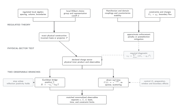
A regulated Hamiltonian and local Hilbert space feed exact constraints or penalty suppression, then a physical sector; a positive transfer-matrix branch and a direct real-time branch meet only at matched renormalized continuum observables, with leakage and positivity failures marked.

Only the branch with a positive transfer operator supports $H=-a_t^{-1}\log T$ and a positive spectral interpretation. Physical-sector projection and Euclidean positivity are independent requirements. The diagram is schematic.

Spectral interpretation and failure modes

For operators on a time slice,

C(t)=\frac{1}{Z}\operatorname{Tr} \left[T^{N_t-t/a_t}OT^{t/a_t}O^\dagger\right] =\sum_n |\langle0\lvert O\rvert n\rangle|^2e^{-(E_n-E_0)t}+\cdots.

Positive weights follow from the Hilbert-space construction. Oscillating signs, negative spectral weights, or complex effective energies can indicate a nonpositive action, an operator spanning multiple time slices, finite temporal boundaries, or a numerical problem. Each must be diagnosed before a mass plateau is interpreted.

The Hamiltonian limit usually holds spatial spacing and couplings fixed while $a_t\to0$ . The renormalized anisotropy must be measured; the bare $a_s/a_t$ is not automatically physical.

Adversarial failure case

Let a symmetric finite transfer matrix have eigenvalues $1$ and $-\varepsilon$ with $0<\varepsilon\ll1$ . Correlators dominated by the first eigenvector can show a clean positive exponential, so a low-energy fit may appear healthy. Nevertheless, the second eigenvector gives $\langle f,Tf\rangle<0$ , and $\log(-\varepsilon)$ is branch dependent and complex: no self-adjoint $H$ satisfies $T=e^{-a_tH}$ . A reflection test basis that spans both modes rejects the construction even when the preferred correlator does not.

Observable-level validation

Test reflection positivity on a basis of half-time observables rather than on one favored correlator.
Check that the finite transfer matrix is symmetric or self-adjoint and has no negative spectral component in the tested sector.
Expand the one-step kernel through the required order in $a_t$ and compare its generator with an independently constructed Hamiltonian.
Verify nonnegative spectral weights and common gaps across at least two time-slice operators.
Measure the renormalized anisotropy and repeat the comparison as $a_t$ changes at fixed spatial regulator.

Common pitfalls

Taking the logarithm of a nonpositive matrix. A formal matrix logarithm can be non-Hermitian or branch dependent. Establish positivity first.

Dropping normalization before identifying ordering terms. Field-dependent measures can turn “constants” into operators. Derive the short-time kernel systematically.

Equating a temporal-continuum limit with the QFT continuum limit. $a_t\to0$ produces a Hamiltonian at fixed spatial regulator. One still needs $a_s\to0$ and $L\to\infty$ .

Learning outcomes

Given a nearest-neighbor Euclidean time-slice kernel, derive its leading Hamiltonian, including normalization or ordering terms, and state the positivity hypotheses used.
Given Euclidean correlator data, identify a negative-weight, temporal-wrap, operator-support, or anisotropy test that determines whether the extracted decay can be interpreted as Hamiltonian spectral data.

Exercises

If $T$ has an eigenvalue $\lambda<0$ , why can no self-adjoint $H$ satisfy $T=e^{-a_tH}$ ?

Solution

The spectral theorem makes $e^{-a_tH}$ strictly positive on every finite-energy eigenvector, with eigenvalues $e^{-a_tE}>0$ . A negative eigenvalue is impossible.

Show that multiplying $T$ by $c>0$ shifts the Hamiltonian by a constant.

References

Section titled “References”- Creutz, M. (1977). Gauge fixing, the transfer matrix, and confinement on a lattice. Physical Review D, 15, 1128–1136. DOI.
- Osterwalder, K., and Seiler, E. (1978). Gauge field theories on a lattice. Annals of Physics, 110, 440–471. DOI.
Further reading
Section titled “Further reading”- Wilson, K. G. (1974). Confinement of quarks. Physical Review D, 10, 2445–2459. DOI.
Original QFT.org content:CC BY 4.0, unless an item supplies different terms. Third-party material retains its own terms.