Contraction, Truncation, and Continuum Error Certification

A tensor-network result is certified by attaching a falsifiable, observable-specific statement to each approximation axis—not by quoting one discarded weight or one smooth bond-dimension curve. Separate the ansatz, optimizer, contraction or environment, time evolution, local Hilbert space, volume, lattice spacing, operator matching, and inference model; then vary them independently or model their correlation explicitly.

Required background. Matrix product states, finite entanglement, and continuum limits supplies transfer and finite-entanglement scales. Tensor renormalization of Euclidean path integrals supplies blocking and contraction errors. Symmetric and gauge-invariant tensor networks supplies exact constraint diagnostics.

Helpful background. PEPS and higher-dimensional field theories supplies approximate environments. Real-time tensor-network dynamics supplies evolution and time-window errors. Complete lattice error budgets supplies covariance and shared-input propagation.

Tensor-network error axes

Write the computed observable with all material controls exposed:

O_{\mathbf c} =O(a,L,d_{\rm loc},\mathcal G,\chi, \chi_{\rm env},r_{\rm opt},\Delta t,t_{\max},Z_O,\ldots).

Here $\mathcal G$ is the ansatz or contraction geometry, $\chi$ the state or blocking bond dimension, $\chi_{\rm env}$ an environment control, $r_{\rm opt}$ an optimizer residual, and $Z_O$ shorthand for operator matching. Not every method uses every entry, but an unused axis must be marked inapplicable rather than silently omitted.

Regulator and convention box. Freeze the target QFT, state or ensemble, observable, renormalization prescription, lattice geometry, and boundary conditions before comparing controls. State every cutoff, dimension, tolerance, initialization, contraction family, fit window, and limit order. Errors sharing tensors, environments, samples, scale setting, or fit inputs are correlated until demonstrated otherwise.

For any chosen sequence of intermediate controls, the difference from a target value can be written as a telescoping identity. For example,

\begin{aligned} O_{a,L,d,\chi,\eta}-O_* ={}&(O_{a,L,d,\chi,\eta}-O_{a,L,d,\chi,\infty})\\ &+(O_{a,L,d,\chi,\infty}-O_{a,L,d,\infty,\infty})\\ &+(O_{a,L,d,\infty,\infty}-O_{a,L,\infty,\infty,\infty})\\ &+(O_{a,L,\infty,\infty,\infty}-O_{a,\infty,\infty,\infty,\infty})\\ &+(O_{a,\infty,\infty,\infty,\infty}-O_*), \end{aligned}

with $\eta$ denoting environment or contraction control. This is bookkeeping, not a claim that the terms are independent or even available separately. Changing the order changes the components when controls interact. Fixed-axis and crossed scans determine whether a useful factorized approximation is defensible.

What each diagnostic can establish

For an exactly evaluated normalized variational state,

E[A]\geq E_0.

This establishes an upper bound on the ground energy, not a bound on a general observable. The residual

r=\|(H-E)|\psi\rangle\|, \qquad r^2=\langle H^2\rangle-E^2,

shows whether the state is close to some eigenstate; converting it into an eigenvector or observable bound needs spectral-separation hypotheses. Approximate PEPS contraction can invalidate the numerical upper-bound statement unless its error is bounded. A local Schmidt discarded weight exactly measures one local Hilbert-norm truncation in its SVD context, but is not a universal bound after nonlinear optimization, repeated truncations, Euclidean blocking, or continuum fitting.

Constraint residuals test the constraints they measure. Energy or norm conservation in real time can coexist with a wrong held-out correlator. Agreement between algorithms sharing the same environment, initialization family, or operator matching is correlated evidence. The evidence label must be no stronger than the weakest consequential axis.

Canonical MPS diagnostics, local truncations, and their domain of interpretation are developed in Schollwöck 2011, §§ 4–5; independent step, projection, and bond controls for time evolution are reviewed in Paeckel et al. 2019, §§ 2–6. The complementary structural treatment of MPS, PEPS, symmetries, and contraction complexity is given by Cirac et al. 2021, §§ II–III and VI, while Orús 2014 develops practical MPS and PEPS constructions and contraction methods.

The joint control map summarizes this logic. Every route to a claim passes fixed-axis scans and a held-out observable; the dashed branch sends a one-axis plateau back to the full control definition.

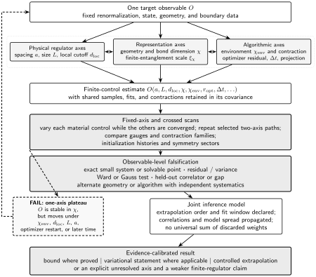
Physical regulator, ansatz, contraction, optimization, and evolution controls feed a common observable; fixed-axis and crossed scans reject a plateau that moves under any untested axis.

Tensor-network uncertainty is joint and observable dependent. The schematic figure requires correlations, alternative models, and unresolved controls to remain explicit; it does not treat discarded weights as universal additive error bars.

Exactly checkable false plateau

Consider the synthetic observable

O(\chi,d)=1+\frac{1}{\chi^2}+\frac{1}{d}.

At fixed $d=8$ , the sequence $\chi=8,16,32$ approaches $1.125$ , and a bond-only fit can look excellent. The target after both limits is $O_*=1$ . A fixed- $\chi=32$ local-space scan gives

O(32,8)=1.1259765625, \quad O(32,16)=1.0634765625, \quad O(32,32)=1.0322265625,

revealing the dominant unresolved axis. This fixture tests whether an analysis pipeline distinguishes a conditional $\chi\to\infty$ intercept from the joint limit. An adversarial extension can add $c\chi/d^2$ to test interactions and fit-order dependence.

Tensor-network regulator and error record

This is the canonical chapter-wide semantic record. Every other method page links here so the table has one maintained instance. A concrete result should fill every row with a value, an uncertainty or bound where justified, and an explicit unresolved limitation where it is not.

Required declarations, falsification tests, and failure signals for a tensor-network QFT result.
Field	Required declaration	Independent test	Failure signal
Target and geometry	Hamiltonian state or Euclidean partition function; lattice, graph, boundaries, sector	Units, orientation, product or exact finite-network limit	State and partition-function networks treated as interchangeable
Physical regulators	Spacing `a`, size `L`, local dimension, bare tuning, limit order	Fixed-axis local-space, volume, and spacing scans	Bond convergence presented as regulator removal
Ansatz and bonds	Tensor class, unit cell or layers, every bond dimension, virtual gauge	Canonical checks, ansatz enlargement, alternate geometry	Area-law compatibility presented as an accuracy theorem
Symmetry and gauge	Irreps, fusion or flux sectors, boundary charge, exact or penalized constraint	Local intertwiner, Ward, and Gauss tests	Exact residual but flux or irrep cutoff still drifting
Contraction and environment	Method, environment dimensions, normalization, tolerances, termination	Frozen-tensor scan and alternate contraction family	Apparent variational bound moves under re-contraction
Optimization	Objective, residual or variance, initialization history, stopping rule	Restarts, tighter tolerance, frozen exact check where available	Sweep plateau with large residual or initialization dependence
Evolution	Integrator, step size, projection, bond-growth rule, maximum time	Step and bond scans; conserved and held-out observables	Smooth trace beyond the first unconverged time
Observable	Insertion, current or composite operator, normalization, matching, units	Sum rule, derivative identity, exact matrix element, alternate insertion	Energy or free energy converges while the target observable drifts
Scan design	Fixed-axis points, crossed points, shared inputs, covariance	Hold each material axis fixed in turn	Only one diagonal cutoff path or unmodeled cancellation
Inference	Asymptotic form, fit window, correction terms, model alternatives	Window changes, held-out cutoff points, residual structure	Exponent or window chosen to recover the desired answer
External benchmark	Exact small system, solvable point, or independent formulation not used in tuning	Freeze choices before comparison	Every comparison participated in optimization or scale setting
Claim boundary	Exact identity, rigorous bound, variational statement, controlled extrapolation, empirical stability, or unresolved	Independent reproduction of the weakest consequential axis	Quoted precision exceeds the least controlled test

Certification protocol

Freeze the target observable and all fitted inputs; designate at least one held-out prediction.
Converge algebraic identities first: tensorization, canonical normalization, isometries, intertwiners, Hermiticity, and constraint signs.
At fixed tensors, converge contraction or environment controls.
At fixed physical regulators, enlarge the ansatz and repeat optimization from independent starts.
Scan $d_{\rm loc}$ , $L$ , and $a$ separately; add crossed points wherever axes visibly interact.
For dynamics, repeat the hierarchy at selected times and stop the reported interval at the earliest failed check.
Propagate shared inputs and fit covariance; vary theoretically allowed asymptotic models and windows.
Compare with an exact or independently controlled result that did not participate in tuning.
Label the conclusion at the weakest supported level and list every open axis.

This sequence is intentionally observable specific. A state may support a precise energy and only a qualitative long-distance correlator; a Euclidean network may support free energy more strongly than a susceptibility; a real-time state may support early local observables but not a late spectral peak.

A reproducible critical-chain calculation must export the completed record, frozen inputs, and independent checks rather than only final plots.

Adversarial failure: correlated agreement

Two PEPS codes agree because both import the same boundary environment and operator normalization. A third optimizer also agrees after minimizing that shared approximate objective. The comparison has three implementations but one dominant systematic. Re-contract frozen tensors with an independent environment, change the operator insertion, and compare an exact small lattice before describing the agreement as cross-method validation.

Observable-level validation checklist

Fill every row of the canonical record, including inapplicable and unresolved fields.
Verify exact identities before numerical extrapolation.
Use fixed-axis scans for every material cutoff and selected crossed scans.
Distinguish variational energies, residual evidence, local discarded weights, and general observables.
Preserve covariance from shared tensors, samples, scale setting, and fit inputs.
Include at least one held-out observable and one adversarial enlargement.
Stop real-time claims at the earliest failed refinement.
Match the observable and repeat the continuum fit under justified alternatives.
State finite-regulator evidence when continuum controls remain open.

What you should be able to do

After this page, you should be able to:

build an observable-specific tensor-network error analysis whose ansatz, optimization, contraction, evolution, local-space, volume, and spacing axes are independently varied or explicitly correlated; and
classify each diagnostic as a rigorous bound, variational statement, asymptotic extrapolation, cross-method test, empirical stability check, or unresolved evidence.

Exercises

1. Conditional intercept. Fit the exact form $O(\chi,8)=A+B/\chi^2$ for the false-plateau fixture. What are $A$ and $B$ , and why is $A$ not the target?

Solution

$A=1+1/8=1.125$ and $B=1$ . The intercept removes the bond regulator only at fixed local dimension $d=8$ ; the remaining $1/d$ term must be extrapolated separately.

2. Evidence class. A normalized, exactly contracted MPS has energy $E$ and residual $r$ , but no known spectral separation. What can be stated safely?

Solution

$E$ is a variational upper bound on the finite-regulator ground energy if the state lies in the correct domain and sector. The residual quantifies failure of the eigenvalue equation. Without spectral separation it does not by itself bound the eigenvector error or a general observable, so those require enlargement and independent checks.

References

Cirac, J. Ignacio, David Pérez-García, Norbert Schuch, and Frank Verstraete. “Matrix Product States and Projected Entangled Pair States: Concepts, Symmetries, Theorems.” Reviews of Modern Physics 93 (2021): 045003. DOI.
Orús, Román. “A Practical Introduction to Tensor Networks: Matrix Product States and Projected Entangled Pair States.” Annals of Physics 349 (2014): 117–158. DOI.
Paeckel, Sebastian, Thomas Köhler, Andreas Swoboda, Salvatore R. Manmana, Ulrich Schollwöck, and Claudius Hubig. “Time-Evolution Methods for Matrix-Product States.” Annals of Physics 411 (2019): 167998. DOI.
Schollwöck, Ulrich. “The Density-Matrix Renormalization Group in the Age of Matrix Product States.” Annals of Physics 326 (2011): 96–192. DOI.