

Light-Front Constraints, Zero Modes, and Vacuum Structure
Constrained field components and longitudinal zero modes obstruct the naive vacuum argument because neither is an independent positive- oscillator. Their equations contain or , whose kernels carry boundary and global data. Solving only the nonzero modes can therefore omit instantaneous interactions, Gauss-law information, order-parameter branches, or topology. Light-front kinematics makes vacuum-to-positive- particle creation impossible under ordinary momentum conservation; it does not prove that the complete physical vacuum is empty.
Required background. Light-Front Coordinates and Quantization supplies the convention, characteristic scalar bracket, and positivity of . Constraints, Dirac Brackets, and Symplectic Reduction supplies the distinction between constraints, gauge conditions, and reduced phase-space brackets.
Helpful background. Vacua, States, and Representations separates a cyclic physical vacuum from a chosen Fock reference state. Symmetry Realization and Order Parameters supplies the infinite-volume and order-parameter criteria used below.
Inverse longitudinal derivatives require boundary data
Section titled “Inverse longitudinal derivatives require boundary data”Convention and regulator card. Coordinates obey and . For explicit constraints, is periodic with length . Every field is split into its average and zero-average part. The symbol acts only on the zero-average part; its kernel is never set to zero by notation. Scalar products at coincident points are regulated and renormalized before the zero-mode projection is taken.
For any periodic field define
Then has zero average, and on Fourier modes ,
There is no entry. Adding an arbitrary function independent of does not change the derivative. A boundary condition or an integrated field equation must determine that function. This elementary kernel is the common source of scalar zero-mode constraints, nondynamical spinor components, and instantaneous gauge interactions.
In infinite volume the same issue reappears as a prescription for the distribution and its endpoint behavior. Periodic finite volume makes the missing mode visible but introduces compactification effects of its own; it is not automatically a Lorentz-invariant infrared regulator. The finite- volume characteristic problem and its causal limitations are analyzed in Heinzl 2000, §§ 3.3–3.5, preprint pp. 24–40, PDF.
The shared map below makes the decisive longitudinal branch explicit: the kernel of leads to a zero-mode constraint and boundary prescription, not to permission to erase the mode. Its other branches show why that constraint must remain coupled to the counterterm and observable tests summarized in the structured regulator table.
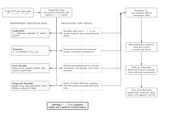
The kernel is a separate constrained sector within the longitudinal regulator branch. The schematic map forbids using positive nonzero to infer an empty physical vacuum and requires the solved constraint to survive matching, symmetry tests, and all relevant limits; it is not to scale.
The interacting scalar zero mode is a constraint
Section titled “The interacting scalar zero mode is a constraint”Consider a real scalar in dimensions with
Its equation of motion is
Write with . Integrating the equation over the box removes the derivative term and gives
This is not an equation of motion in for an independent oscillator. It is a nonlinear operator constraint that relates to the nonzero modes. In the quantum theory, the cubic composite requires a regulator, an ordering prescription, and the same counterterms as the Hamiltonian. Solving the bare classical polynomial and inserting it into an unrenormalized quantum Hamiltonian is not a controlled approximation. Constrained scalar zero modes and their perturbative and nonperturbative solutions are treated in Brodsky, Pauli, and Pinsky 1998, § 7A, arXiv PDF pp. 126–136.
For the free massive theory, and imply . That exactly checkable result tests the projection and signs. It does not license setting the zero mode to zero after interactions or a different potential are introduced.
A classical broken-potential benchmark
Section titled “A classical broken-potential benchmark”Replace the potential by
For an -independent classical configuration, the exact integrated constraint is
with branches
Deleting the zero mode erases the two nonzero stationary branches before any dynamics is solved. Keeping them still does not prove spontaneous symmetry breaking in the quantum theory: at finite volume, tunneling and the definition of the state matter, while a broken phase requires an order parameter and a specified infinite-volume/source limit. The benchmark demonstrates a lost possibility, not a final vacuum selection.
This distinction is central to the light-front literature. Positivity of constrains the oscillator Fock expansion, while nontrivial vacuum physics may be encoded in constrained zero modes or effective Hamiltonian operators Burkardt 1996, §§ 3–4, pp. 17–39. Detailed realizations depend on the theory and regulator; they are not a universal theorem that every condensate is “inside a hadron” or that every light-front vacuum is trivial.
Fermions have good and constrained components
Section titled “Fermions have good and constrained components”Let
The component contains the independent light-front spinor data. In light-front gauge , projection of the Dirac equation gives, schematically but with the normalization explicit,
Thus
The last term is the undetermined kernel component. Substituting the solution back into the Hamiltonian produces interactions nonlocal in ; in gauge theory it also couples to residual constraints. The free-field decomposition, including which spinor component is dynamical, is derived in Hiller 2016, § 2.2.2, preprint pp. 6–8, PDF.
Calling “nondynamical” means it is fixed by a constraint once the boundary problem is complete. It does not mean it may be discarded. Doing so changes mass terms, helicity-flip interactions, currents, and Ward identities.
Gauge constraints generate instantaneous interactions
Section titled “Gauge constraints generate instantaneous interactions”In a gauge such as , not all components of carry independent data. Gauss’s law determines a longitudinal component through an equation containing . Substitution yields an instantaneous interaction with the structural form
where the coefficient, sign, color contraction, residual-gauge term, and zero-mode subtraction depend on the declared theory and convention. The formula is deliberately structural: it shows why the pole prescription and zero-mode sector must accompany the Hamiltonian. Gauge-field constraints and instantaneous fermion and gauge-boson terms are worked out in Brodsky, Pauli, and Pinsky 1998, §§ 2A–2H, arXiv PDF pp. 12–34.
Residual gauge transformations independent of survive the local condition . Global Gauss-law constraints, boundary charges, and Wilson lines can therefore remain. A calculation must state its residual gauge condition and physical-state constraint; a formal inverse cannot do that work.
Vacuum statements have a precise ceiling
Section titled “Vacuum statements have a precise ceiling”For interactions that conserve and contain only strictly positive- creation operators, the empty oscillator state cannot mix with a state of positive total . The warranted statement is:
The positive-momentum Fock vacuum is an eigenstate of the regulated Hamiltonian in the sector where all zero-mode, boundary, and constraint contributions have been separately resolved.
It is stronger than an equal-time perturbative mnemonic and weaker than “the physical vacuum is empty.” A vacuum or symmetry claim additionally needs:
- the constraint and its branches;
- the order of source, volume, and regulator limits;
- a gauge-invariant or otherwise physical order parameter;
- agreement of charges, Ward identities, and the low-energy spectrum; and
- a translation to an independent formulation when equivalence is asserted.
Maskawa and Yamawaki’s finite-volume analysis isolates the constrained zero mode and demonstrates why it cannot be inferred from the positive modes alone Maskawa and Yamawaki 1976, pp. 270–283. Subsequent light-front symmetry-breaking analyses also show that the charge, current, and zero-mode limits must be handled together Yamawaki 1998, §§ 1–3, arXiv PDF pp. 7–40.
Adversarial failure: the projected equation is never formed
Section titled “Adversarial failure: the projected equation is never formed”Take the broken-potential scalar model, omit from the mode expansion, and diagonalize only positive modes. The matrix can converge beautifully as its positive-mode basis grows. Yet every vector in that sequence satisfies by construction, so the calculation cannot test the nonzero branches of the exact integrated constraint. Convergence inside the wrong projected space is not evidence that the omitted sector is irrelevant.
The repair is observable: solve or parameterize the zero-mode constraint, repeat the spectrum and order-parameter calculation under admissible boundary prescriptions, and compare a held-out quantity. If the branch or observable changes beyond the error target, the vacuum claim fails.
Observable-level validation
Section titled “Observable-level validation”- Constraint residuals: evaluate the integrated scalar equation, projected Dirac equation, and Gauss law on every computed state.
- Kernel dependence: vary the longitudinal boundary condition or allowed zero-mode prescription while holding the renormalized target fixed.
- Symmetry: test charge conservation, the relevant Ward identity, and degeneracies or Goldstone behavior only after stating finite-volume limitations.
- Instantaneous terms: verify cancellation or combination with propagating contributions in a physical amplitude or current matrix element.
- Cutoff separation: vary , harmonic resolution, small- cutoff, transverse cutoff, and Fock-sector cutoff independently.
- Independent benchmark: reproduce the free constraint , the classical stationary branches above, or a matched equal-time/Euclidean observable before making an interacting claim.
You should now be able to (1) solve a simple scalar or fermion constraint while displaying the kernel and boundary datum, and (2) reject a trivial-vacuum argument that deletes the very sector in which symmetry, topology, or Gauss data may reside. The resulting dynamical amplitudes continue in Light-Front Fock Space, Wavefunctions, and Bound-State Equations. General spontaneous symmetry breaking remains with Symmetry Realization and Order Parameters, and theorem-level null-surface algebra belongs to Mathematical QFT.
Exercises
Section titled “Exercises”Solve a constrained fermion mode
Section titled “Solve a constrained fermion mode”In the free -dimensional theory with and no transverse momentum, use to find and recover the mass shell from the dynamical equation .
Solution
With the phase , , so . Substitute this into the dynamical equation: . Hence . The calculation cannot be repeated at because the constraint cannot be inverted there.
Diagnose the missing broken branches
Section titled “Diagnose the missing broken branches”For the classical potential , compute on all three constant solutions and explain what a basis with can and cannot decide.
Solution
At , . At ,
The two nonzero stationary configurations are classically lower. A basis that fixes cannot compare them and therefore cannot decide vacuum selection. Conversely, the classical comparison alone does not establish quantum spontaneous symmetry breaking at finite volume; the quantum state and limit order remain to be specified.
References
Section titled “References”- Brodsky, Stanley J., Hans-Christian Pauli, and Stephen S. Pinsky. 1998. “Quantum Chromodynamics and Other Field Theories on the Light Cone.” Physics Reports 301: 299–486. DOI. Open PDF.
- Burkardt, Matthias. 1996. “Light Front Quantization.” Advances in Nuclear Physics 23: 1–74. DOI. Open PDF.
- Heinzl, Thomas. 2001. “Light-Cone Quantization: Foundations and Applications.” In Methods of Quantization, Lecture Notes in Physics 572, 55–142. DOI. Open PDF.
- Hiller, John R. 2016. “Nonperturbative Light-Front Hamiltonian Methods.” Progress in Particle and Nuclear Physics 90: 75–124. DOI. Open PDF.
- Maskawa, Toshihide, and Koichi Yamawaki. 1976. “The Problem of Mode in the Null-Plane Field Theory and Dirac’s Method of Quantization.” Progress of Theoretical Physics 56: 270–283. DOI.
- Yamawaki, Koichi. 1998. “Zero-Mode Problem on the Light Front.” DPNU-98-07, arXiv:hep-th/9802037, 63 pp. arXiv DOI. Open PDF.
Original QFT.org content:CC BY 4.0, unless an item supplies different terms. Third-party material retains its own terms.