Lattice Perturbation Theory, Symanzik Analysis, and Improvement

Lattice perturbation theory expands the declared finite-spacing action, measure, and operators themselves. Its propagators and vertices are periodic functions of momenta, and every loop integral runs over a compact Brillouin zone. Matching compares renormalized quantities in a named lattice and continuum scheme. The resulting coefficients enter the Symanzik effective action and operator expansion, where exact regulator symmetries determine the allowed cutoff terms. Improvement is successful only when the predicted leading power is absent from held-out observables across several spacings.

Required background. Lattice Momentum, Propagators, and Cutoff Dispersion supplies lattice kernels and Brillouin zones. Bare Parameters, Tuning Conditions, and Continuum Targets fixes the target trajectory. Relevant, Marginal, and Irrelevant Directions supplies the RG classification.

Helpful background. Momentum-Space Feynman Rules and Anatomy of a Loop Integral provide continuum diagrammatics. Representation and Spurion Constraints on Operator Bases and Symmetry-Protected Operators, Currents, and Improvement supply basis and current constraints.

Lattice Feynman rules come from the regulated action

Use the two-dimensional Euclidean scalar fixture

$$S=a^2\sum_x\left[ \sum_{\mu=1}^2\frac{(\phi_{x+a\hat\mu}-\phi_x)^2}{2a^2} +\frac12m_0^2\phi_x^2 +\frac{\lambda}{4!}\phi_x^4 \right].$$

Define dimensionless variables

$$k_\mu=ap_\mu, \qquad \widehat m=am_0, \qquad \widehat\lambda=a^2\lambda, \qquad \widehat k^2=4\sum_{\mu=1}^2\sin^2\!\left(\frac{k_\mu}{2}\right).$$

In lattice units the free propagator and quartic vertex are

$$G_0(k)=\frac1{\widehat k^2+\widehat m^2}, \qquad V_4=-\widehat\lambda,$$

with momentum conservation modulo $2\pi$ in each component. The vertex sign is the coefficient in the expansion of $e^{-S_{\mathrm{int}}}$; a different convention for amputated Euclidean vertices must be translated consistently.

Perturbative conventions. The page uses a Euclidean weight $e^{-S}$, incoming lattice momenta in $[-\pi,\pi]^2$, the site-wide conventions, and the dimensionless action above. The lattice action, field measure, gauge-fixing and ghost terms when present, operator basis, continuum target scheme, scale $\mu$, and infrared regulator are local. Continuum $k^2$ must never replace $\widehat k^2$ inside a lattice loop.

At one loop, the tadpole self-energy has symmetry factor $1/2$:

$$\widehat\Sigma_{\mathrm{lat}}^{(1)} =\frac{\widehat\lambda}{2}I_{\mathrm{lat}}(\widehat m), \qquad I_{\mathrm{lat}}(\widehat m) =\int_{[-\pi,\pi]^2}\frac{\mathrm d^2k}{(2\pi)^2} \frac1{\widehat k^2+\widehat m^2}.$$

The domain, measure, propagator, vertex, and symmetry factor are inseparable parts of the rule. In gauge theory, expansion of link variables and the Haar measure adds vertices; gauge fixing and ghosts must be derived from the lattice formulation rather than copied from the continuum.

A bounded one-loop matching coefficient

The scalar integral has the exact representation

$$I_{\mathrm{lat}}(\widehat m) =\frac{2}{\pi(4+\widehat m^2)} K\!\left(\frac4{4+\widehat m^2}\right),$$

where the complete elliptic integral uses the modulus convention

$$K(k)=\int_0^{\pi/2} \frac{\mathrm d\theta}{\sqrt{1-k^2\sin^2\theta}}.$$

Libraries that accept the parameter $k^2$ require an explicit conversion. As $\widehat m\to0$,

$$I_{\mathrm{lat}}(\widehat m) =-\frac1{4\pi}\log\widehat m^2 +\frac{\log32}{4\pi} +O(\widehat m^2\log\widehat m^2).$$

In two-dimensional $\overline{\mathrm{MS}}$ at $\mu=1/a$, the corresponding subtracted tadpole is

$$I_{\overline{\mathrm{MS}}} =-\frac1{4\pi}\log\widehat m^2.$$

Therefore the finite lattice-to-$\overline{\mathrm{MS}}$ coefficient is

$$C_{\mathrm{lat}\to\overline{\mathrm{MS}}} =\lim_{\widehat m\to0} \left[I_{\mathrm{lat}}-I_{\overline{\mathrm{MS}}}\right] =\frac{\log32}{4\pi} =0.2757945001908145\ldots.$$

With the self-energy convention above,

$$m_{\overline{\mathrm{MS}}}^2-m_{0,\mathrm{lat}}^2 =\frac\lambda2 C_{\mathrm{lat}\to\overline{\mathrm{MS}}}, \qquad \frac{a^2\Delta m^2}{\widehat\lambda} =\frac{C}{2} =0.1378972500954073\ldots.$$

This is a complete matching benchmark because the lattice integral, continuum subtraction, scale, action, and symmetry factor are fixed. The coefficient is not universal: changing the lattice action or continuum scheme changes its finite part.

Numerical evaluation should compare four independent routes: periodic quadrature over the Brillouin zone, adaptive integration, the elliptic formula, and the small-mass extrapolation. Grid error, adaptive error, special-function convention, asymptotic-fit error, and floating-point error remain separate. Taking $\widehat m=0$ in either infrared-divergent integral before forming the difference is invalid.

Symanzik action and operator expansions

For momenta and masses well below $1/a$, a local lattice theory can be represented by a continuum effective action

$$\mathcal L_{\mathrm{Sym}} =\mathcal L_{\mathrm{target}} +\sum_i a^{\Delta_i-d}c_i(a\mu,g_R) \mathcal Q_i,$$

and a lattice operator by

$$\mathcal O_{\mathrm{lat}} =\sum_j Z_j(a\mu)\mathcal O_{R,j}(\mu) +\sum_k a^{\Delta_k-\Delta_{\mathcal O}} d_k(a\mu)\mathcal R_k(\mu).$$

The bases contain every local operator allowed by the exact lattice symmetries, boundary conditions, and quantum numbers. Lower-dimensional mixings belong in the first matching problem, not in a positive-power cutoff expansion. Logarithms can multiply powers of $a$ through anomalous dimensions.

Terms proportional to the leading equations of motion can be removed by field redefinitions for on-shell observables under suitable boundary conditions. They may still matter for off-shell Green functions, contact terms, boundary observables, and a fixed operator definition. “Redundant” must therefore state the observable class.

For the standard free scalar,

$$\widehat p^2 =p^2-\frac{a^2}{12}\sum_\mu p_\mu^4+O(a^4),$$

so the leading bulk artifact is represented by a hypercubic dimension-$d+2$ operator. A five-point Laplacian can cancel its tree-level coefficient, but temporal next-nearest-neighbor terms require a separate reflection-positivity check. Boundary and anisotropic lattices admit additional localized or direction-dependent operators.

Symanzik’s construction and improvement conditions are developed in the original two-part analysis Symanzik 1983, Part I, pp. 187–204 and Part II, pp. 205–227. Lattice power counting provides conditions under which continuum renormalization and lattice integrals have the expected asymptotic structure Reisz 1988.

Coefficient determination and improvement tests

Improvement coefficients can be determined perturbatively, nonperturbatively from Ward identities or matching conditions, or by a hybrid method. The condition used to tune a coefficient is not an independent test. Reserve observables with different kinematics or operator content.

Suppose an unimproved dimensionless observable has

$$R(a)=R_0+c_2(a\Lambda)^2+c_4(a\Lambda)^4+\cdots,$$

and the leading coefficient is canceled. The improved prediction is

$$R_{\mathrm{imp}}(a)=R_0+c_4'(a\Lambda)^4+\cdots$$

only if no other $O(a^2)$ action, operator, mass-dependent, boundary, or mistuning term survives. Testing requires multiple spacings spanning an asymptotic window, common physical volume and masses, and a comparison of $a^2$ versus $a^4$ residual models. A small coefficient over one interval is weaker than the predicted power law.

On-shell improvement of an action does not automatically improve a composite operator. The action changes energies and states; the operator expansion changes matrix elements. Both must be treated for a precision observable.

Adversarial failure cases

Continuum propagator inside the Brillouin zone. Replacing $\widehat k^2$ by $k^2$ changes the regulator and the finite matching coefficient.

Tadpole factor lost. The $1/2$ is a graph symmetry factor. Numerical agreement after retuning another convention does not repair a missing factor.

Scale changed without RG conversion. The displayed $\overline{\mathrm{MS}}$ comparison uses $\mu=1/a$. Another $\mu$ changes the logarithm and must be evolved.

Power divergence invented in the two-dimensional fixture. The matched difference is logarithmic and finite. Dimensional analysis and the exact elliptic result rule out an uncanceled $1/a^2$ term here.

One improved observable. A coefficient tuned on one dispersion point can overfit it. Test other momenta, directions, and an operator matrix element.

Off-shell and on-shell improvement conflated. Equation-of-motion operators may drop from one class and remain in another.

The chain below distinguishes a matched improvement coefficient from the continuum claim it helps to control. Inspect how the action, operator basis, scheme, scale, and cutoff ansatz remain linked, and how an alternative action or held-out observable supplies an independent test.

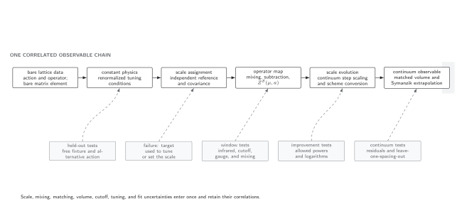
A continuum prediction requires a tuned bare trajectory and a renormalized observable. Scale, matching, mixing, volume, and cutoff uncertainties remain separate and correlated; held-out checks test rather than define the trajectory. The diagram is schematic and not to scale.

Observable-level validation checklist

Before claiming matching or improvement, require:

• propagators, vertices, measures, and conservation deltas derived from the exact lattice action;
• compact Brillouin-zone loop domains and lattice momentum symbols;
• all gauge-fixing, ghost, Haar-measure, and operator-insertion terms when applicable;
• a named continuum scheme, scale, infrared prescription, and basis translation;
• symmetry factors and dimensions checked independently;
• exact, quadrature, and asymptotic routes agreeing for a bounded fixture;
• a symmetry-complete Symanzik action and operator basis;
• tunable and equation-of-motion-redundant terms separated by observable class;
• multiple matched spacings and held-out observables showing the predicted residual power; and
• perturbative truncation, nonperturbative tuning, and continuum-fit uncertainties kept distinct.

Any implementation of the exact tadpole fixture must reproduce $\log32/(4\pi)$ before making a broader matching claim.

Exercises

1. Tadpole symmetry factor. Expand $e^{-\widehat\lambda\sum_x\phi_x^4/4!}$ to first order and contract two fields at the vertex with two external fields. Show that the self-energy coefficient is $\widehat\lambda/2$.

Solution

There are $4\times3=12$ ways to attach the two labeled external fields, leaving the remaining two fields to contract with each other. Dividing by $4!=24$ gives $12/24=1/2$. The minus sign from the Euclidean interaction expansion is incorporated in the vertex convention; the mass correction has the displayed positive loop coefficient in the inverse propagator.

2. Directional improvement test. Why must equal-$p^2$ on-axis and diagonal momenta be included when testing cancellation of the $a^2p^{[4]}$ term?

Solution

The continuum term depends only on $p^2$, while the hypercubic artifact depends on $p^{[4]}$. Equal-$p^2$ directions isolate the breaking coefficient without changing the target kinematics. A fit using only on-axis momenta cannot distinguish a rotationally invariant $a^2(p^2)^2$ term from the hypercubic one.

What you can now do

You should now be able to derive lattice Feynman rules, evaluate and independently check a compact-zone matching integral, construct the allowed Symanzik action and operator basis, and test improvement through residual scaling. Continue with Lines of Constant Physics and Continuum Extrapolation to combine tuning, scale, renormalization, volume, and these cutoff predictions in one correlated limit.

References

• Reisz, Thomas. “A Power Counting Theorem for Feynman Integrals on the Lattice.” Communications in Mathematical Physics 116, no. 1 (1988): 81–126. doi:10.1007/BF01239027.
• Symanzik, Kurt. “Continuum Limit and Improved Action in Lattice Theories. I. Principles and $\phi^4$ Theory.” Nuclear Physics B 226, no. 1 (1983): 187–204. doi:10.1016/0550-3213(83)90468-6.
• Symanzik, Kurt. “Continuum Limit and Improved Action in Lattice Theories. II. O($N$) Nonlinear Sigma Model in Perturbation Theory.” Nuclear Physics B 226, no. 1 (1983): 205–227. doi:10.1016/0550-3213(83)90469-8.

References

Section titled “References”- Guttmann, Anthony J. “Lattice Green Functions in All Dimensions.” Journal of Physics A: Mathematical and Theoretical 43, no. 30 (2010): 305205. doi:10.1088/1751-8113/43/30/305205.
- OpenAI Codex for QFT.org. “Lattice Observables and Continuum Inference Benchmark.” JavaScript source, validated 25 August 2026. SHA-256
d76924d8c724cb7c9307fb38265336495fa3ff1a98103b3fa4fa734262647c2a. Reproducibility record. - Reisz, Thomas. “A Power Counting Theorem for Feynman Integrals on the Lattice.” Communications in Mathematical Physics 116, no. 1 (1988): 81–126. doi:10.1007/BF01239027.