Anatomy of a Loop Integral

A loop integral is defined by considerably more than a drawn graph. One must specify its denominators and powers, numerator, independent loop variables, external momenta, masses, integration measure, regulator, and causal boundary value. Those data determine not only its value but also where ultraviolet, infrared, and threshold singularities can arise.

Required background. Momentum-Space Feynman Rules supplies the rule that turns internal lines, vertices, and momentum conservation into propagator denominators and numerators.

Helpful background. Lorentzian Boundary Conditions and the $i\epsilon$ Prescription explains why the sign of the infinitesimal imaginary part selects the Feynman boundary value.

The data carried by an L-loop integral

For scalar propagators, a useful family notation is

$$I(\boldsymbol\nu;\{p\},\{m\})= \mu^{2L\epsilon} \int\prod_{r=1}^{L}\frac{\mathrm d^d\ell_r}{(2\pi)^d}\, \frac{N(\ell,p)}{\prod_{j=1}^{n} \bigl(q_j^2-m_j^2+i0\bigr)^{\nu_j}}, \qquad d=4-2\epsilon .$$

Here each internal momentum is an affine combination

$$q_j=\sum_{r=1}^{L}c_{jr}\ell_r+P_j(\{p\}),$$

with integer incidence coefficients $c_{jr}$ and an external-momentum combination $P_j$. A zero index $\nu_j$ pinches that denominator; a negative index places the corresponding inverse propagator in the numerator. Irreducible scalar products not spanned by the chosen inverse propagators remain in $N$. For spinning fields, $N$ can also contain Lorentz, spinor, color, and gauge-dependent data; it cannot be inferred from the denominator topology.

The definition must also record the orientation of external momenta, the physical or complex kinematic point, and any conventional prefactor such as $e^{\gamma_E\epsilon}(4\pi)^{-\epsilon}$. Different prefactors merely reshuffle Laurent coefficients, but comparing results without stating them creates false disagreements. A systematic momentum-space definition and the role of its $i0$ boundary value are developed in Weinzierl 2022, §2.4.2, pp. 28–39; §2.5.1, pp. 41–42.

Routing and translation invariance

A different graph routing replaces $\ell_r$ by an integer linear combination of loop momenta plus external momenta. For the usual unimodular routing changes, a translation-invariant regulator makes this an ordinary change of variables and leaves the regulated integral unchanged. Dimensional regularization has this property. A sharp cutoff centered at $\ell=0$ generally does not: shifting $\ell$ moves the integration boundary, so a superficially divergent integral can acquire a surface term. Weinzierl 2022, §2.4.2, pp. 28–39 states the dimensional-continuation conventions used here.

This matters whenever an algebraic Ward identity uses a shift such as

$$\int \mathrm d^d\ell\,[f(\ell+p)-f(\ell)]=0.$$

The equation is legitimate only after the integral has been defined in a shift-invariant scheme, or after the regulator-dependent surface contribution has been accounted for. “Symmetric integration” is not a substitute for this check.

Where singular behavior can originate

Power counting first examines a common large rescaling $\ell_r\mapsto\Lambda\ell_r$. If the numerator has loop-momentum degree $R$, the superficial degree for that scaling is

$$\omega=Ld+R-2\sum_j\nu_j.$$

$\omega\ge 0$ signals a possible ultraviolet divergence, not a proof: tensor contractions, gauge identities, or subdivergences can alter the conclusion. Each independent subgraph scaling must also be tested.

Infrared singularities instead come from finite-momentum boundaries where massless denominators become small. A soft region has every component of a loop momentum small. A collinear region can have large energy but small virtuality because it aligns with a lightlike external direction. Threshold behavior is different again: poles in loop energy approach the contour from opposite sides and prevent its deformation. The integral may then develop a branch point even though no loop momentum is large or uniformly small.

For the bubble, write $E_1(\boldsymbol\ell)=\sqrt{\boldsymbol\ell^2+m_1^2}$ and $E_2(\boldsymbol\ell)=\sqrt{(\boldsymbol\ell+\mathbf p)^2+m_2^2}$. A pole below the real $\ell^0$ axis at $\ell^0=E_1-i0$ meets a pole above it at $\ell^0=p^0-E_2+i0$ when

$$p^0=E_1+E_2.$$

In the center-of-mass frame the minimum is $p^0=m_1+m_2$, hence $p^2=(m_1+m_2)^2$. This energy-contour check is independent of the UV degree and explains why a fully massive bubble can be infrared finite yet nonanalytic at threshold.

The figure summarizes these distinct scaling questions. Inspect especially the unequal component scaling in a collinear or potential region and the separate contour-pinch test.

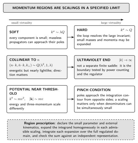
Momentum regions are homogeneous scalings relative to a declared small parameter, not universal pieces of every integral. The diagram is schematic and not to scale; the collinear components use light-cone coordinates, and the potential scaling applies near a nonrelativistic threshold.

An equivalent diagnostic is:

Candidate source	Limiting behavior	Necessary check
UV	one or more independent loop momenta become large	subgraph power counting and regulator
Soft IR	a massless momentum tends uniformly to zero	whether adjacent denominators simultaneously approach shell
Collinear IR	momentum becomes parallel to a lightlike external leg	component scaling and numerator suppression
Threshold	internal energies can become simultaneously on shell	pole locations and contour pinching
Potential	$k^0\sim mv^2$, $	\mathbf k

The general integral data, parametric representation, and scale properties are reviewed in Abreu, Britto, and Duhr 2022, §1, pp. 3–8.

A bubble normalization check

For

$$B(p^2)=\mu^{2\epsilon}\int\frac{\mathrm d^d\ell}{(2\pi)^d} \frac{1}{(\ell^2-m_1^2+i0)((\ell+p)^2-m_2^2+i0)},$$

the measure has mass dimension $d$, while two propagators contribute $-4$; hence $[B]=d-4=-2\epsilon$ before the factor $\mu^{2\epsilon}$ and zero afterward. At large $\ell$, the integrand scales as $d^d\ell/\ell^4$, so the four-dimensional UV behavior is logarithmic. For nonzero masses and off-shell Euclidean $p^2<0$, soft and collinear singularities are absent. A physical branch point can nevertheless occur after continuation to $p^2=(m_1+m_2)^2$.

This one example already separates three notions often conflated: UV power counting, IR endpoint behavior, and a finite-momentum threshold pinch.

Exercises

1. Under $\ell\mapsto\ell-p$, verify that the bubble denominators exchange their routing roles after relabeling the masses. The Jacobian is one; equality still presumes a translation-invariant regulator.
2. For a rank-two numerator $N=\ell^\mu\ell^\nu$, find the superficial degree in four dimensions. Here $R=2$, so $\omega=2$: covariance and reduction may lower particular coefficients, but naive convergence cannot be assumed.

Where the integral data are used

• Feynman and Schwinger Parameters turns the declared denominators and prescription into a parameter-domain geometry.
• Landau Equations and Physical Singularities tests which finite-momentum on-shell configurations can actually pinch a contour.

References

• Abreu, Samuel, Ruth Britto, and Claude Duhr. “The SAGEX Review on Scattering Amplitudes, Chapter 3: Mathematical Structures in Feynman Integrals.” Journal of Physics A: Mathematical and Theoretical 55 (2022): 443004. doi:10.1088/1751-8121/ac87de.
• Weinzierl, Stefan. Feynman Integrals. Cham: Springer, 2022. doi:10.1007/978-3-030-99558-4. Open PDF.