Positive Geometry and Canonical Forms

A positive geometry is an oriented semialgebraic domain in a suitable real slice of an algebraic variety for which a unique rational top form exists with recursively prescribed boundary residues and no other singularities. In special amplitude problems, this boundary structure can package locality and factorization. The canonical-form statement is exact for a geometry satisfying the definition; identifying a proposed geometry with a QFT amplitude is a separate, theory-specific claim.

Required background. Leading Singularities and Integrand Geometry supplies multidimensional residues and the distinction between integrand data and integrated amplitudes.

Canonical forms from boundaries

At orientation level, a $d$-dimensional positive geometry is a pair $(X,X_{\ge0})$, where $X$ is an irreducible complex projective variety of complex dimension $d$ and $X_{\ge0}\subset X(\mathbb R)$ is a nonempty, oriented, closed semialgebraic set of real dimension $d$, subject to the boundary regularity assumptions in the definition. Its nonzero rational canonical top form $\Omega(X_{\ge0})$ is characterized recursively by:

1. only logarithmic singularities on the boundaries;
2. no other singularities;
3. residue on each boundary equal, with induced orientation, to that boundary’s canonical form.

For the interval $a<x<b$,

$$\Omega_{[a,b]} =\frac{(b-a)\,\mathrm dx}{(x-a)(b-x)} =\mathrm d\log\frac{x-a}{b-x}.$$

It has simple logarithmic poles at the two endpoints. For the affine triangle

$$x>0, \qquad y>0, \qquad 1-x-y>0,$$

the canonical form is

$$\Omega_\triangle =\frac{\mathrm dx\wedge\mathrm dy}{x\,y\,(1-x-y)}.$$

Taking the residue at $x=0$ gives, up to the induced orientation,

$$\operatorname*{Res}_{x=0}\Omega_\triangle =\frac{\mathrm dy}{y(1-y)},$$

the interval form on that edge. This is the recursive principle in its simplest explicit form.

The figure shows the triangle, its three logarithmic boundary factors, and the residue descent from the two-form to an edge one-form and then a vertex. No color encodes the relation.

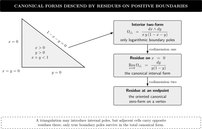
Boundary recursion for the canonical form of a positive triangle. Each codimension-one boundary is a logarithmic pole, and its residue is the canonical form of that edge; a further residue reaches a vertex. The construction is exact for the displayed simplex and the diagram is schematic rather than metric.

The general definition, uniqueness, and triangulation properties are developed in Arkani-Hamed, Bai, and Lam 2017, §§ 2–4, pp. 5–11; simplex and amplituhedron examples continue in Arkani-Hamed, Bai, and Lam 2017, §§ 5–7.2, pp. 12–51.

Triangulations and spurious boundaries

Suppose a positive geometry is decomposed into oriented cells $C_r$ with disjoint interiors. Canonical forms add:

$$\Omega(X_{\ge0})=\sum_r\Omega(C_r).$$

Boundaries internal to the triangulation appear with opposite orientations in adjacent cells, so their poles cancel. This is analogous to cancellation of spurious poles among amplitude terms: the decomposition is representation dependent, while the total canonical form is invariant.

For the interval, splitting at $c$ gives

$$\Omega_{[a,b]} =\Omega_{[a,c]}+\Omega_{[c,b]}.$$

Each term has a pole at $x=c$, but the residues cancel. This provides a direct algebraic check that a triangulation has not introduced a physical boundary.

A four-point interval encodes two channels

The simplest amplitude check uses the massless planar biadjoint scalar tree with ordering $[1234\mid1234]$. Strip the coupling, color factors, momentum-conserving delta function, and overall amplitude phase. With all momenta outgoing, let

$$s=(p_1+p_2)^2, \qquad t=(p_2+p_3)^2, \qquad u=(p_1+p_3)^2, \qquad s+t+u=0.$$

Choose $c>0$ and restrict to the auxiliary positive slice

$$u=-c, \qquad s\ge0, \qquad t=c-s\ge0.$$

This is not physical real Lorentzian phase space; it is the oriented interval $0\le s\le c$. Pulling back its canonical form gives

$$\begin{aligned} \Omega(\mathcal A_4) &=\frac{\mathrm ds}{s}-\frac{\mathrm ds}{s-c}\\ &=\frac{\mathrm ds}{s}+\frac{\mathrm ds}{t} =\mathrm d\log\frac{s}{t}. \end{aligned}$$

Thus the rational coefficient in the $\mathrm ds$ basis is

$$m_4[1234\mid1234]=\frac1s+\frac1t,$$

the two planar factorization channels in the declared stripped normalization. Near $s=0$ the oriented residue is $+1$. Near $t=0$, the positive coordinate is $t=c-s$, so $\mathrm ds=-\mathrm dt$ and the one-form residue is $-1$, even though the rational $t$-channel coefficient is $+1$. This distinction between boundary orientation and channel coefficient is essential. The four-point associahedron pullback is derived in Arkani-Hamed et al. 2018, § 3.3, printed p. 17, PDF.

Amplitudes in a bounded domain

The physical $m=4$ amplituhedron is a theory-specific construction for color-ordered, planar, four-dimensional $\mathcal N=4$ supersymmetric Yang–Mills data. It is labeled by particle number $n$, helicity sector $k$, and loop order $L$, and it requires positive external data in momentum-twistor variables. The proposal identifies its canonical form with the $n$-particle N$^k$MHV tree superamplitude or $L$-loop integrand. The original paper explicitly classified that identification as a conjecture supported by nontrivial checks, rather than a theorem for arbitrary $n,k,L$ Arkani-Hamed and Trnka 2014, § 1, pp. 2–4; §§ 9–11, pp. 17–22. In sectors where a triangulation reproduces BCFW recursion, the match supplies a constructive verification Arkani-Hamed, Bai, and Lam 2017, § 7.2.3, pp. 43–45.

Several qualifications are essential:

• the construction uses four-dimensional planar ordering, $\mathcal N=4$ supersymmetry, a declared $(n,k,L)$ sector, and positive external data;
• the canonical object is naturally an integrand or differential form, not automatically a regulated integrated amplitude;
• different triangulations can resemble different expansion terms while introducing spurious internal boundaries that cancel only in the sum;
• positivity and the map from geometric variables to kinematic data must be specified;
• extensions to other theories, dimensions, or nonplanar sectors are separate constructions, not consequences of the original definition.

The frontier evidence table marks the canonical-form property as definitional for positive geometries satisfying the recursive axioms and the amplituhedron–amplitude identification as a theory-specific construction. Its evidence cutoff is 9 August 2026; this page does not infer a universal amplitude geometry from the cited planar construction.

Factorization and leading singularities

If a physical codimension-one boundary corresponds to a propagator invariant $P^2\to0$, then after pulling back to compatible local coordinates a logarithmic form can behave schematically as

$$\Omega\sim\frac{dP^2}{P^2}\wedge\Omega_L\wedge\Omega_R.$$

Its residue then factorizes into lower-dimensional canonical forms, mirroring amplitude factorization. The displayed relation suppresses the sum over intermediate states or its superspace measure, projective weights, and theory-dependent normalization. Higher-codimension intersections encode iterated residues and can match leading singularities.

This parallel must be checked, not assumed. A geometric boundary can be spurious under a map, and an amplitude singularity may require data not represented by a chosen geometry. Integrated branch cuts and infrared regularization also go beyond a rational integrand’s boundary form.

Validation workflow

For a proposed amplitude geometry:

1. define the ambient space, positive region, orientation, and map to kinematics;
2. enumerate all boundary components and their physical interpretation;
3. verify that the proposed form has only logarithmic poles on those boundaries;
4. compute residues and match the induced boundary forms and factorization normalizations;
5. triangulate in at least two ways and confirm internal poles cancel;
6. compare representative leading singularities or low-point amplitudes;
7. state whether the result is an integrand, a regulated differential form, or an integrated observable.

Common pitfalls

Calling any positive integration region a positive geometry. The recursive canonical-form property and boundary stratification are essential parts of the definition.

Treating triangulation poles as physical. Internal cell boundaries must cancel in the sum. Check residues, not only denominators.

Equating an integrand form with an integrated amplitude. Regulators, contours, branch cuts, and boundary conditions enter integration.

Generalizing the amplituhedron without restating its domain. Planarity, supersymmetry, external data, and kinematic sector are not optional details.

Exercises

Split the interval $[a,b]$ at $c$ and write the two canonical forms explicitly. Show that the internal residues cancel.

Solution

The two forms are

$$\begin{aligned} \Omega_{[a,c]} &=\frac{\mathrm dx}{x-a}-\frac{\mathrm dx}{x-c},\\ \Omega_{[c,b]} &=\frac{\mathrm dx}{x-c}-\frac{\mathrm dx}{x-b}. \end{aligned}$$

Their $x=c$ poles have coefficients $-1$ and $+1$. Adding the forms cancels that spurious boundary and gives

$$\Omega_{[a,b]} =\frac{\mathrm dx}{x-a}-\frac{\mathrm dx}{x-b} =\frac{(b-a)\,\mathrm dx}{(x-a)(b-x)}.$$

Where to continue

• Leading Singularities and Integrand Geometry develops the residue data used in the comparison.
• S-Matrix and Amplitude Bootstrap uses factorization and analyticity without presupposing a positive geometry.
• Color–Kinematics Duality contains the shared evidence table.

References

• Arkani-Hamed, Nima, Yuntao Bai, Song He, and Gongwang Yan. “Scattering Forms and the Positive Geometry of Kinematics, Color and the Worldsheet.” Journal of High Energy Physics 05 (2018): 096, esp. § 3.3. doi:10.1007/JHEP05(2018)096. Open PDF.
• Arkani-Hamed, Nima, and Jaroslav Trnka. “The Amplituhedron.” Journal of High Energy Physics 10 (2014): 030. doi:10.1007/JHEP10(2014)030. Open PDF.
• Arkani-Hamed, Nima, Yuntao Bai, and Thomas Lam. “Positive Geometries and Canonical Forms.” Journal of High Energy Physics 11 (2017): 039. doi:10.1007/JHEP11(2017)039. Open PDF.