Momentum-Space Feynman Rules

Momentum-space Feynman rules are the Fourier transform of the quadratic kernel and interaction monomials in a declared action. In the all-momenta-incoming convention, invert the regulated quadratic kernel for each internal line, multiply each interaction coefficient by $i$ and by the momentum factors generated by derivatives, impose a momentum-conserving delta distribution at every vertex, integrate each independent internal momentum with $\mathrm d^d\ell/(2\pi)^d$, and divide by the graph symmetry factor. This procedure fixes signs and normalizations without relying on a memorized model catalog.

Required background. Diagrammatics and Symmetry Factors supplies the decorated graphs and their residual factors.

Helpful background. Fourier Series, Fourier Transforms, and Plancherel Theory supplies the transform and convolution rules; Scalar Propagators, Ordered Correlators, and Sources fixes the Feynman boundary value.

Quadratic kernels become propagators

Write a bosonic quadratic action in momentum space as

$$S_0 =\frac12\int\frac{\mathrm d^d p}{(2\pi)^d}\, \phi_A(-p)K^{AB}(p)\phi_B(p).$$

The internal-line rule is the regulated inverse

$$D_{AB}(p)=i\,[K(p)+i0\,\mathcal B]^{-1}_{AB},$$

where $\mathcal B$ abbreviates the state and boundary prescription needed for the particular kernel. For a canonically normalized real scalar,

$$K(p)=p^2-m^2, \qquad D_F(p)=\frac{i}{p^2-m^2+i0}.$$

This is not merely algebraic matrix inversion at a pole: the $+i0$ boundary value is part of the propagator. Constrained or gauge-degenerate quadratic forms must be gauge fixed or reduced before they can be inverted.

For a Dirac field with

$$\mathcal L_0=\bar\psi(i\gamma^\mu\partial_\mu-m)\psi,$$

the same Fourier convention gives the inverse kernel $p\!\!\!/-m$ and

$$S_F(p) =\frac{i(p\!\!\!/+m)}{p^2-m^2+i0}.$$

Multiplication by $p\!\!\!/-m$ returns $i$ away from the prescribed pole, providing an immediate numerator and sign check.

Local interactions become vertices

With

$$\phi(x)=\int\frac{\mathrm d^d p}{(2\pi)^d} e^{-ip\cdot x}\widetilde\phi(p),$$

the spacetime integral of a local product produces

$$\int\mathrm d^d x\, e^{-i(p_1+\cdots+p_n)\cdot x} =(2\pi)^d\delta^{(d)}\!\left(\sum_{j=1}^{n}p_j\right).$$

Thus a conventionally normalized interaction

$$\mathcal L_{\mathrm{int}} =-\frac{\lambda_n}{n!}\phi^n$$

gives the vertex

$$-i\lambda_n(2\pi)^d \delta^{(d)}\!\left(\sum_{j=1}^{n}p_j\right).$$

The $n!$ has already been canceled by the identical field attachments. If the action does not contain that factorial, the vertex rule must retain the corresponding combinatorial multiplicity. Momentum-space conversion and the vertex delta functions are worked explicitly in Schwartz 2014, § 7.3, pp. 93–99 and Weinberg 1995, § 6.3, pp. 281–285.

Exact vertex momentum conservation uses translation invariance. If a coupling is switched, $\lambda_n\to\lambda_n g(x)$, the same Fourier transform gives $\widetilde g(p_1+\cdots+p_n)$ rather than a delta distribution. The delta is recovered only when the constant-coupling or infinite-volume limit exists; it should not be imposed prematurely in finite-time calculations.

Derivatives act on the field immediately following them and produce $-ip_\mu$ for an incoming momentum $p$. For example,

$$\mathcal L_{\mathrm{int}} =-\frac g2\chi\,\partial_\mu\phi\,\partial^\mu\phi$$

gives, with both identical $\phi$ momenta incoming,

$$V_{\chi\phi\phi}(p_\chi,p_1,p_2) =ig\,p_1\cdot p_2, \qquad p_\chi+p_1+p_2=0.$$

The sign follows mechanically: each derivative gives $-ip$, the action contributes $i$, and the two identical $\phi$ attachments cancel the explicit $1/2$. Derivative Interactions and Contact Terms treats the integration-by-parts and time-derivative qualifications.

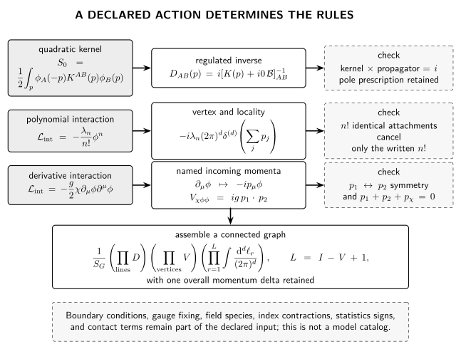
The action-to-rule map is summarized below. Inspect which data are algebraic and which remain prescriptions.

From action terms to momentum-space ingredients in the site Fourier convention. The quadratic kernel is inverted only after its boundary or gauge prescription is fixed; polynomial factorials determine identical-field combinatorics; each derivative supplies $-ip_\mu$ on its own incoming field. The diagram is schematic and does not replace model-specific index contractions.

Action datum	Momentum-space rule	Independent check
$\frac12\phi K\phi$	$i(K+i0\,\mathcal B)^{-1}$	multiplying by $K$ gives $i$ as a distributional inverse
$-\lambda_n\phi^n/n!$	$-i\lambda_n$	direct Wick counting cancels $n!$
one local spacetime integral	$(2\pi)^d\delta^{(d)}(\sum p)$	translation invariance conserves momentum
$\partial_\mu\phi$	$-ip_\mu\widetilde\phi(p)$	a total derivative gives $-i\sum p_\mu=0$ at the vertex
closed independent momentum cycle	$\int\mathrm d^d\ell/(2\pi)^d$	$L=I-V+1$ for a connected graph

Assemble a connected graph

For a connected graph $G$ with $I$ internal lines and $V$ vertices:

1. assign an incoming momentum to every half-edge;
2. put one propagator on each internal line;
3. put the complete tensor and coupling factor on each vertex;
4. include one delta distribution per vertex;
5. integrate one momentum per internal line;
6. use $V-1$ independent vertex deltas to perform integrals, retaining one overall delta; and
7. multiply by $1/S_G$ and all statistics signs.

The number of remaining integrals is

$$L=I-(V-1)=I-V+1,$$

the number of independent loops in a connected graph. After stripping the overall delta, a tree has $L=0$ and therefore no unconstrained loop integration. Weinberg derives this counting directly from the vertex delta functions Weinberg 1995, § 6.3, pp. 282–283.

In compressed notation the contribution therefore has the structure

$$\mathcal G_G(\{p\})= \frac{(2\pi)^d\delta^{(d)}(\sum p)}{S_G} \int\prod_{r=1}^{L}\frac{\mathrm d^d\ell_r}{(2\pi)^d} \prod_{e\in E_{\mathrm{int}}}D_e(q_e) \prod_{v\in V}V_v(\{q\}_v),$$

with a declared routing $q_e(\{p\},\{\ell\})$. A change of loop routing is a change of integration variables only when the regulator respects that shift; superficially divergent integrals require care before such manipulations are used.

As a minimal check, the one-vertex $\phi^4$ connected four-point function contributes

$$(2\pi)^d\delta^{(d)}(p_1+p_2+p_3+p_4)(-i\lambda) \prod_{j=1}^{4}\frac{i}{p_j^2-m^2+i0}$$

before amputation. There is one vertex delta, no internal line, and no loop integral. The external propagators belong to the correlator; LSZ later removes them under stable-particle pole assumptions.

Overall factors and convention checks

Several conventions can change the appearance of intermediate rules:

• choosing all momenta outgoing replaces every displayed incoming momentum by its negative;
• defining a propagator without its numerator factor $i$ moves powers of $i$ elsewhere;
• changing the sign of $\mathcal L_{\mathrm{int}}$ changes the vertex sign; and
• reversing an oriented fermion or ghost line changes which momentum is named incoming, not the final invariant amplitude.

A reliable translation reconstructs a simple correlator from the action and checks its pole, residue, momentum delta, and mass dimension. “Up to conventions” is not enough when an amplitude sign or phase is at stake.

Common pitfalls

Inverting a singular gauge kernel. A gauge-invariant quadratic form has null directions. Declare the gauge-fixed action first; its inverse is gauge dependent and is not itself an observable.

Adding an extra factorial at the vertex. The factorial in a normalized interaction monomial is designed to cancel identical attachments. Count from the written action once.

Integrating every internal momentum after using deltas. Start with one integral per internal line, then use independent vertex deltas. A connected graph retains exactly $L=I-V+1$ loop variables.

Check your understanding

Starting from $\mathcal L_{\mathrm{int}}=-g\chi\phi^2/2$, derive the three-point vertex, including its momentum delta and identical-field factor.

Solution

Fourier transforming the three fields gives one spacetime exponential $e^{-i(p_\chi+p_1+p_2)\cdot x}$, hence $(2\pi)^d\delta^{(d)}(p_\chi+p_1+p_2)$. The perturbative expansion contributes $i(-g/2)$, while the two identical $\phi$ fields can be attached in $2!$ ways. The factors cancel, leaving

$$-ig(2\pi)^d\delta^{(d)}(p_\chi+p_1+p_2).$$

Where to continue

• Track graded signs: Fermion Signs and Closed Loops fixes open-line ordering and loop signs.
• Handle momentum-dependent vertices carefully: Derivative Interactions and Contact Terms separates spatial derivatives from time-ordering contact terms.
• Convert correlators into stable-particle amplitudes: Asymptotic States, LSZ, and Scattering Observables supplies external residues, amputation, and state normalization.

References

• Schwartz, Matthew D. Quantum Field Theory and the Standard Model. Cambridge: Cambridge University Press, 2014. DOI.
• Weinberg, Steven. The Quantum Theory of Fields, Volume I: Foundations. Cambridge: Cambridge University Press, 1995. First edition; 2005 paperback, 2012 printing consulted. DOI.