Soft Theorems

When one emitted massless quantum has energy much smaller than every hard invariant, its leading amplitude separates into a universal soft current times the amplitude without that quantum. The pole comes from attaching the emission to external on-shell lines. Its residue knows their momenta and charges but, at leading power, not the short-distance details of the hard interaction.

Required background. Soft and Collinear Singularities supplies the on-shell denominator $1/(p\cdot k)$ and defines the soft limit used below.

Helpful background. Asymptotic Symmetry, Soft Limits, and the Boundary Interface relates soft identities to boundary charges. That reinterpretation is not needed for the amplitude derivation here.

The leading gauge-theory soft factor

Let $k$ and $\varepsilon(k)$ be the momentum and polarization of an additional outgoing gluon, and suppose $k^0=\omega\to0$ while all hard invariants stay fixed and nonzero. Write the collection of hard momenta as $\{p\}_n$. At tree level,

$$\begin{aligned} \mathcal M_{n+1}^{a}(\{p\}_n;k) ={}&g_s\,\varepsilon_\mu^*(k)J_a^\mu(k)\\ &\times\mathcal M_n(\{p\}_n)+O(\omega^0), \end{aligned}$$

In a physical-momentum convention, write

$$J_{a,\mathrm{phys}}^\mu(k)= \sum_{i=1}^{n}\eta_i\,\mathbf t_i^a \frac{p_i^\mu}{p_i\cdot k}.$$

Here $p_i$ denotes a future-directed physical momentum, $\eta_i=+1$ for an outgoing hard leg and $-1$ for an incoming one, and $\mathbf t_i^a$ is the generator carried by the corresponding physical particle, with no crossing sign absorbed. Equivalently, cross every hard leg to an all-outgoing momentum $\widehat p_i=\eta_i p_i$ and let $\mathbf T_i^a$ denote the image of $\eta_i\mathbf t_i^a$ under the corresponding crossing map of the amplitude’s leg space. For an incoming non-Abelian leg this map includes passage to the conjugate representation and the appropriate transpose; it is not merely a scalar sign on an unchanged matrix. Because $\widehat p_i^\mu/(\widehat p_i\cdot k)=p_i^\mu/(p_i\cdot k)$, the same current is

$$J_{a,\mathrm{out}}^\mu(k) =\sum_i\mathbf T_i^a\frac{\widehat p_i^\mu} {\widehat p_i\cdot k}.$$

The symbols $\mathbf t_i$ and $\mathbf T_i$ must not be mixed: the explicit $\eta_i$ belongs to the physical-momentum convention, while orientation and conjugation are already contained in the all-outgoing crossed charge. In QED, where the charge is a number, this reduces to $Q_i^{\mathrm{out}}=\eta_iQ_i$. The formula is valid away from additional collinear or multiparticle singular limits.

Catani and Grazzini give the color-space soft current and its squared correlations in Catani and Grazzini 2000, § 2, printed pp. 2–5, PDF. Weinberg derives the corresponding photon and graviton poles in Weinberg 1965, pp. B516–B521.

Why only external lines supply the pole

For a scalar external leg, emission after the hard interaction contains

$$\begin{aligned} &g_s\mathbf t_i^a(2p_i+k)^\mu \frac{1}{(p_i+k)^2-m_i^2+i0}\\ &\qquad=g_s\mathbf t_i^a \frac{p_i^\mu}{p_i\cdot k+i0}+O(\omega^0). \end{aligned}$$

For a fermion, the numerator algebra and on-shell Dirac equation give the same leading spin-independent factor. An incoming attachment has the crossed orientation and opposite $i0$ prescription. An internal hard line remains off shell by an order-$Q^2$ invariant under a generic soft perturbation, so its attachment begins at $O(\omega^0)$. This argument fails if the purported hard process is already at another on-shell pinch; the simultaneous limit must then be factorized as a multiparticle region rather than as an isolated soft theorem.

The same replacement by a classical ray is displayed below. Inspect the orientation of each ray: it fixes both the color generator and the causal prescription of the eikonal denominator.

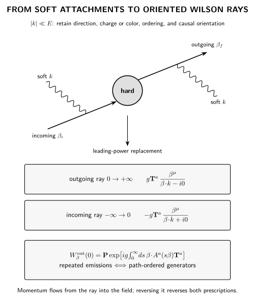
Leading soft emission sees an energetic particle only through its direction $\beta$, charge or color generator, and incoming or outgoing orientation. Repeated attachments are ordered along the corresponding Wilson ray. The diagram is schematic and does not represent a complete process-specific soft function.

The Ward check fixes the charge sum

Replacing the soft polarization by its momentum gives

$$k_\mu J_{a,\mathrm{phys}}^\mu(k) =\sum_i\eta_i\mathbf t_i^a.$$

Gauge invariance therefore requires

$$\left(\sum_i\eta_i\mathbf t_i^a\right)\mathcal M_n=0,$$

or, after applying the crossing maps to all leg spaces,

$$\left(\sum_i\mathbf T_i^a\right)\mathcal M_n^{\mathrm{out}}=0.$$

This is precisely color conservation of the hard amplitude. In QED it is ordinary charge conservation. Thus the leading soft theorem passes its Ward test only after attachments to every charged external leg are included. The test also fixes relative signs that cannot be inferred from the absolute value of a rate.

For more than one soft gluon, the generators do not commute. Successive emissions are ordered along each hard direction, and correlated non-Abelian terms enter when comparable soft energies are taken together. Iterating a single-emission factor without specifying a strong energy ordering is not the general multi-soft theorem.

Gravity and the limits of the comparison

For a soft outgoing graviton with symmetric polarization $\varepsilon^*_{\mu\nu}$, the leading tree expression is

$$\begin{aligned} \mathcal M_{n+1}^{\mathrm{grav}} ={}&\frac{\kappa}{2}\,\varepsilon^*_{\mu\nu}(k) \sum_i\eta_i\frac{p_i^\mu p_i^\nu}{p_i\cdot k}\\ &\times\mathcal M_n+O(\omega^0). \end{aligned}$$

The replacement $\varepsilon_{\mu\nu}\to k_{(\mu}\xi_{\nu)}$ reduces to momentum conservation rather than charge conservation. This is a structural comparison, not a claim that all gauge and gravity soft corrections coincide.

Subleading $O(\omega^0)$ and sub-subleading terms can involve angular momentum operators, spin, recoil, and derivatives of the hard amplitude. Their universality depends more strongly on dimension, particle content, loop order, and how simultaneous infrared limits are taken. Loop soft currents can also contain additional infrared poles. Low’s theorem controls the first terms for photon emission under its analyticity assumptions (Low 1958, pp. 974–977); it should not be promoted without qualification to an arbitrary non-Abelian or gravitational loop statement.

Check your understanding

Contract the gauge-theory current with $k_\mu$. Check that the denominators cancel before using any kinematic approximation beyond $k^2=0$. Then repeat for the graviton factor and verify that the gauge variation vanishes by $\sum_i\eta_i p_i^\mu=0$. Finally, identify why either check fails if one hard external leg is omitted.

References

• Catani, Stefano, and Massimiliano Grazzini. “The Soft-Gluon Current at One- Loop Order.” Nuclear Physics B 591 (2000): 435–454, esp. § 2, printed pp. 2–5 of the author manuscript. doi:10.1016/S0550-3213(00)00572-1. Open PDF.
• Low, Francis E. “Bremsstrahlung of Very Low-Energy Quanta in Elementary Particle Collisions.” Physical Review 110 (1958): 974–977. doi:10.1103/PhysRev.110.974.
• Weinberg, Steven. “Infrared Photons and Gravitons.” Physical Review 140 (1965): B516–B524. doi:10.1103/PhysRev.140.B516.